How to Build a Salmon Index and Quantify Bulk RNA-Seq Reads
Aligning 45 million reads to a genome sounds rigorous. For RNA-seq quantification, it is often unnecessary.
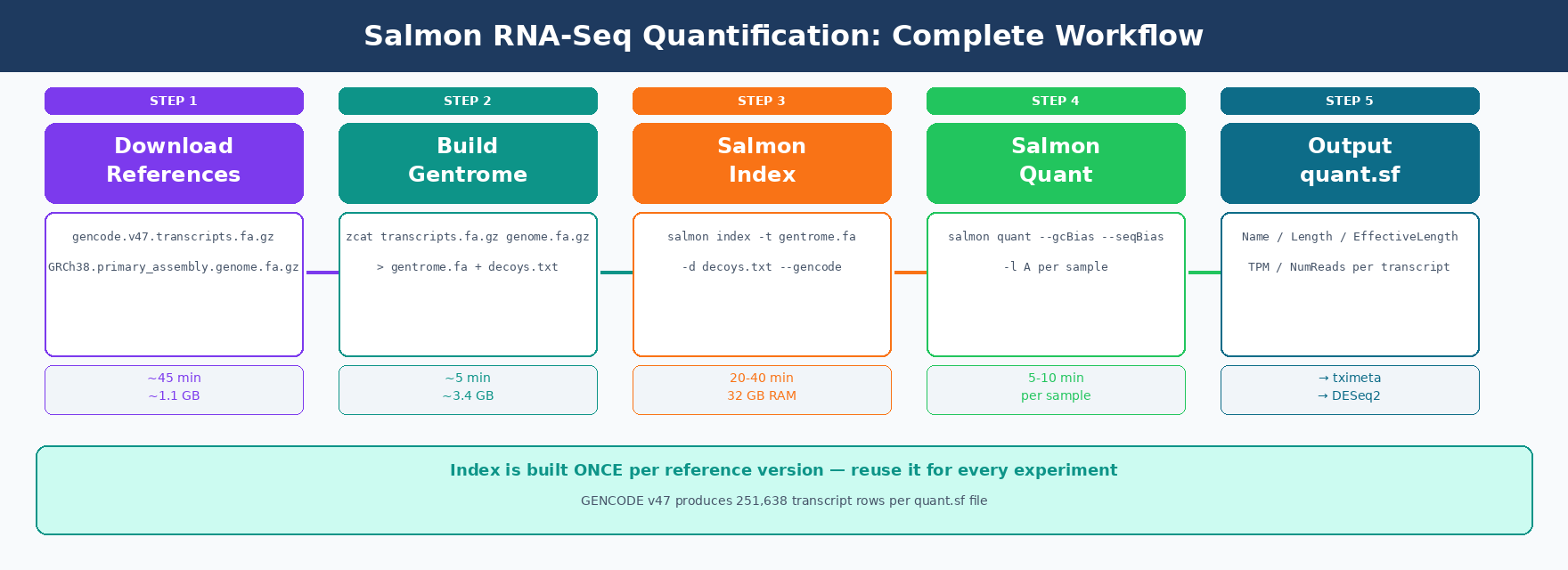
Salmon takes your trimmed reads, maps them directly to the transcriptome, and produces transcript-level abundance estimates in minutes per sample. No BAM files. No coordinate-sorted outputs. Just a quant.sf file per sample, ready for DESeq2 or tximeta.
This post covers the complete Salmon workflow: downloading the GENCODE reference, building a decoy-aware index, running salmon quant on all samples with bias correction, and checking your mapping rates before moving to differential expression.
We continue from the FASTQ quality control tutorial. Your trimmed FASTQ files live in results/trimmed/.
Why Use Salmon Instead of STAR + featureCounts
Both approaches produce gene-level counts, but they take different paths.
STAR aligns reads to the full genome and produces BAM files. featureCounts then assigns those reads to genes. The genome index alone requires 38 GB of RAM for human data.
Salmon maps reads directly to the transcriptome using selective alignment. It needs about 8 GB of RAM. It runs 5-10x faster than alignment-based methods and skips intermediate BAM files entirely.
The tradeoff is that Salmon is transcript-aware, not genome-aware. It does not tell you where in the genome a read came from. If you need genome-level alignments for visualization in IGV or for structural variant calling, use STAR. For differential expression from counts, Salmon is the faster and equally accurate choice.
Salmon is the first quantifier to correct for GC content bias
Salmon was introduced in Patro et al. 2017 in Nature Methods as the first transcriptome-wide quantifier to correct for fragment GC content bias. The paper demonstrated this substantially improves accuracy of abundance estimates and the reliability of subsequent differential expression analysis.
How to Download the GENCODE Reference Files for Human RNA-Seq
The Salmon index needs two files: the transcript sequences (FASTA) and the primary genome assembly (also FASTA, used as decoy).
We use GENCODE as our reference. It provides comprehensive human gene annotations with consistent transcript IDs across releases.
# Create a reference directorymkdir -p references && cd references
# ── GENCODE human v47 ────────────────────────────────────────────────# 1. Transcript sequences (needed for the Salmon index)wget "https://ftp.ebi.ac.uk/pub/databases/gencode/Gencode_human/release_47/gencode.v47.transcripts.fa.gz"
# 2. Primary genome assembly (used as decoy sequences)wget "https://ftp.ebi.ac.uk/pub/databases/gencode/Gencode_human/release_47/GRCh38.primary_assembly.genome.fa.gz"
# 3. GTF annotation (used later for tximeta and for QC)wget "https://ftp.ebi.ac.uk/pub/databases/gencode/Gencode_human/release_47/gencode.v47.annotation.gtf.gz"
echo "Reference downloads complete."ls -lh
Storage: these files are large
The transcript FASTA is about 250 MB compressed. The genome FASTA is about 900 MB compressed but expands to 3.1 GB uncompressed. The combined gentrome used for indexing will be around 3.4 GB. The final Salmon index directory is about 2-4 GB. Plan for at least 15 GB of free disk space in this directory.
For mouse experiments, swap the GENCODE human URL for the mouse equivalent.
# Mouse (GRCm39, GENCODE vM34)wget "https://ftp.ebi.ac.uk/pub/databases/gencode/Gencode_mouse/release_M34/gencode.vM34.transcripts.fa.gz"wget "https://ftp.ebi.ac.uk/pub/databases/gencode/Gencode_mouse/release_M34/GRCm39.primary_assembly.genome.fa.gz"How to Build a Decoy-Aware Salmon Index
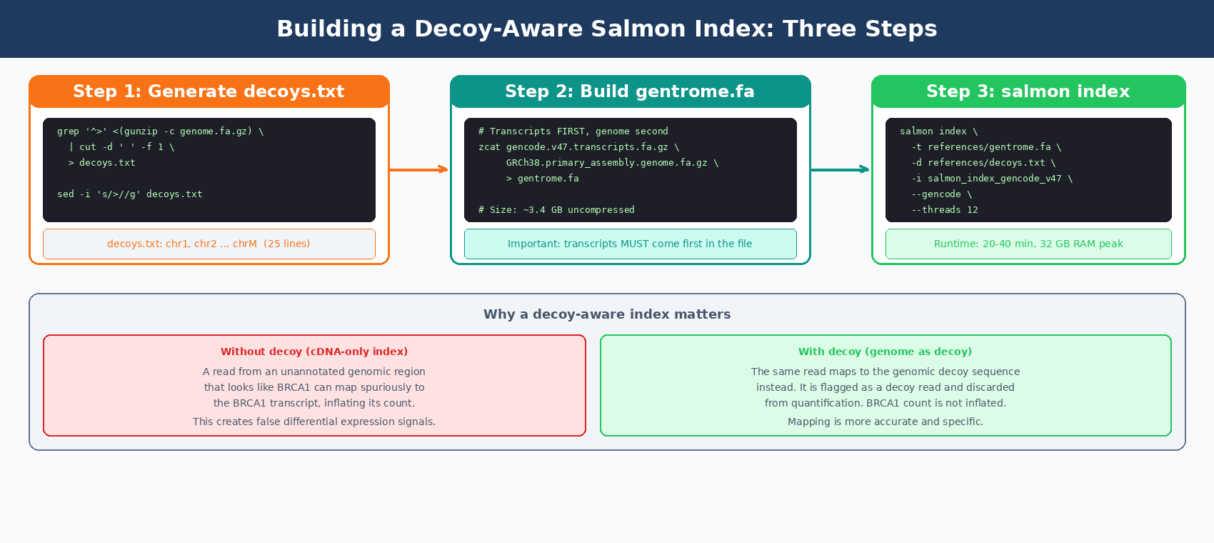
A plain Salmon index maps reads only against transcripts. A decoy-aware index also contains genomic sequences that act as a sink for reads that arise from unannotated genomic regions and would otherwise map spuriously to annotated transcripts.
Salmon recommends using selective alignment with a decoy-aware transcriptome to mitigate potential spurious mapping of reads that arise from some unannotated genomic locus that is sequence-similar to an annotated transcriptome.
We build the “full genome as decoy” version. It produces the most accurate results and avoids running the computationally expensive MashMap step.
Step 1: Build the decoys.txt file
This file lists the chromosome names from the genome FASTA. Salmon uses it to know which sequences are decoys versus transcripts.
cd references
# Extract chromosome names from the genome FASTAgrep "^>" <(gunzip -c GRCh38.primary_assembly.genome.fa.gz) \    | cut -d " " -f 1 \    > decoys.txt
# Remove the leading ">" from each namesed -i 's/>//g' decoys.txt
# Check the outputhead -5 decoys.txt# chr1# chr2# chr3# chr4# chr5
wc -l decoys.txt  # Should be ~25 for GRCh38 primary assembly
Step 2: Build the gentrome (transcript + genome combined FASTA)
Salmon requires the transcripts to come first, genome sequences second.
# Concatenate transcriptome first, then genome# This takes ~5 minutes and produces a 3.4 GB filezcat gencode.v47.transcripts.fa.gz \     GRCh38.primary_assembly.genome.fa.gz \     > gentrome.fa
echo "gentrome.fa size:"du -sh gentrome.fa# ~3.4G    gentrome.fa
Step 3: Build the Salmon index
cd ..   # back to the project root
salmon index \    --transcripts references/gentrome.fa \    --decoys       references/decoys.txt \    --index        references/salmon_index_gencode_v47 \    --gencode \    --threads 12 \    --kmerLen 31
echo "Index complete."ls -lh references/salmon_index_gencode_v47/
The --gencode flag is required when using GENCODE FASTA files. Without it, Salmon cannot parse the pipe-delimited transcript IDs in GENCODE headers correctly.
The index build takes 20-40 minutes and uses about 32 GB of RAM at peak. It only needs to run once per reference version.
How to Run salmon quant on Paired-End RNA-Seq Reads
With the index built, quantification is straightforward. Each sample needs one salmon quant command.
Quantify one sample first
Run one sample to check that the setup is working before running all of them.
mkdir -p results/quant
salmon quant \    --index    references/salmon_index_gencode_v47 \    --libType  A \    --mates1   results/trimmed/SRR26891234_1.trimmed.fastq.gz \    --mates2   results/trimmed/SRR26891234_2.trimmed.fastq.gz \    --gcBias \    --seqBias \    --threads  8 \    --output   results/quant/SRR26891234_quant \    2>&1 | tee logs/salmon_SRR26891234.log
Salmon prints a live summary as it runs. You should see the library type it detected and a running mapping rate. A healthy mapping rate is above 80%.
[info] Automatically detected most likely library type as ISF[info] Processed 45,123,456 total fragments[info] Mapping rate = 92.41%What each flag does
--libType A tells Salmon to automatically detect the library strandedness. This works correctly for almost all modern RNA-seq protocols. Salmon will print what it detected.
--gcBias enables GC content bias correction at the fragment level. Running Salmon with --gcBias in any case is fine, as it does not impair quantification for samples without GC bias, it just takes a few more minutes per sample.
--seqBias corrects for sequence-specific bias caused by random hexamer priming, the same effect that causes the per-base sequence content FAIL in FastQC.
Both bias flags are independent. Using both is the recommended practice for any standard poly-A RNA-seq library.
How to Quantify All Samples in Parallel with a Batch Script
For a full experiment, run all samples with a single script.
#!/bin/bash# Run salmon quant on all trimmed paired-end samples
set -euo pipefail
INDEX="references/salmon_index_gencode_v47"TRIMDIR="results/trimmed"QUANTDIR="results/quant"LOGDIR="logs"THREADS=8
mkdir -p "$QUANTDIR" "$LOGDIR"
for R1 in "$TRIMDIR"/*_1.trimmed.fastq.gz; do    sample=$(basename "$R1" _1.trimmed.fastq.gz)    R2="$TRIMDIR/${sample}_2.trimmed.fastq.gz"
    echo "[$(date +%H:%M:%S)] Quantifying $sample"
    salmon quant \        --index   "$INDEX" \        --libType A \        --mates1  "$R1" \        --mates2  "$R2" \        --gcBias \        --seqBias \        --threads "$THREADS" \        --output  "$QUANTDIR/${sample}_quant" \        2>&1 | tee "$LOGDIR/salmon_${sample}.log"
    echo "[$(date +%H:%M:%S)] Done: $sample"done
echo "All samples quantified. Results in $QUANTDIR"
Run it:
bash salmon_quant_all.shEach sample takes 5-10 minutes with 8 threads. A 12-sample experiment finishes in about 1-2 hours running sequentially. If you have enough RAM, you can run 2-3 samples in parallel using GNU parallel.
# Parallel version: 3 samples at a time, 4 threads eachls results/trimmed/*_1.trimmed.fastq.gz | \parallel -j 3 \ 'sample=$(basename {} _1.trimmed.fastq.gz); \ salmon quant \ --index references/salmon_index_gencode_v47 \ --libType A \ --mates1 {} \ --mates2 results/trimmed/${sample}_2.trimmed.fastq.gz \ --gcBias --seqBias --threads 4 \ --output results/quant/${sample}_quant \ 2>&1 | tee logs/salmon_${sample}.log'How to Verify Salmon Output: Mapping Rates and quant.sf
After each sample finishes, Salmon writes a directory with multiple files. The most important are quant.sf and logs/salmon_quant.log.
ls results/quant/SRR26891234_quant/# aux_info/ ← model files used for bias correction# cmd_info.json ← exact command that was run (useful for reproducibility)# lib_format_counts.json ← evidence for library type detection# logs/ ← detailed run logs# quant.sf ← the counts file you needThe quant.sf file
This tab-separated file has one row per transcript.
head -5 results/quant/SRR26891234_quant/quant.sfName Length EffectiveLength TPM NumReadsENST00000456328.2|... 1657 1208.41 0.032145 0.890ENST00000450305.2|... 632 189.71 0.000000 0.000ENST00000488147.1|... 1351 856.36 0.094821 1.863ENST00000419779.2|... 466 51.22 0.000000 0.000The NumReads column is the one DESeq2 uses after tximeta/tximport converts transcript-level estimates to gene-level counts.
Extracting mapping rates across all samples
After running all samples, collect the mapping rates into a summary table.
# Extract mapping rate from each salmon logecho -e "sample\tmapping_rate" > results/quant/mapping_rates.tsv
for logfile in logs/salmon_*.log; do    sample=$(basename "$logfile" .log | sed 's/salmon_//')    rate=$(grep "Mapping rate" "$logfile" | grep -oP '[0-9]+\.[0-9]+')    echo -e "${sample}\t${rate}%" >> results/quant/mapping_rates.tsvdone
cat results/quant/mapping_rates.tsv
Expected output:
sample mapping_rateSRR26891234 92.41%SRR26891235 91.88%SRR26891236 93.12%SRR26891240 90.55%SRR26891241 91.34%SRR26891242 92.09%What mapping rates tell you
A mapping rate above 80% is generally acceptable. Above 85% is good. Above 90% is excellent for most human datasets.
A sample with a mapping rate below 70% is a serious problem. Common causes are using the wrong reference organism, heavy rRNA contamination, using --libType incorrectly, or giving Salmon untrimmed reads.
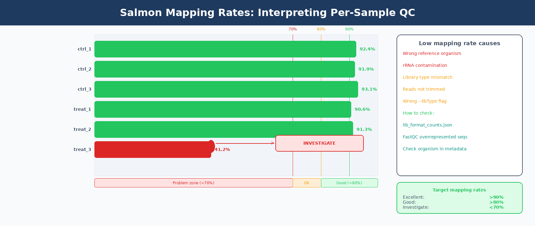
Check lib_format_counts.json if mapping rate is unexpectedly low
Salmon writes a lib_format_counts.json file inside each output directory. It shows how many reads were classified under each possible library orientation. If the winning category has only slightly more reads than the second place, Salmon may have inferred the wrong library type. Try running with the explicit library type: ISR for standard stranded Illumina, IU for unstranded.
How to Run MultiQC on Salmon Outputs
MultiQC reads the Salmon log files and adds mapping rate, detected library type, and quantified fragment counts to the existing QC report.
# Add Salmon results to the existing MultiQC reportmultiqc \ results/fastqc_raw/ \ results/fastqc_trimmed/ \ results/quant/ \ --outdir results/multiqc/ \ --filename "full_QC_report.html" \ --title "RNA-seq QC + Salmon Quantification Summary"The updated report now includes a “Salmon” section showing per-sample mapping rates in a bar chart. It is the fastest way to spot any sample whose mapping rate is an outlier.
What Comes Next: Loading quant.sf into DESeq2
Each sample now has a quant.sf file. The next step is loading these into R using tximeta (which automatically attaches transcript coordinates from GENCODE) or tximport for a simpler import.
The import step requires a transcript-to-gene mapping file so that transcript-level TPMs can be summarized to gene-level counts. We cover this in the DESeq2 walkthrough in R and the PyDESeq2 walkthrough in Python.
For now, verify that all your quant.sf files exist and are non-empty.
# Quick check: all samples have a quant.sf filefor sample_dir in results/quant/*/; do sf="${sample_dir}quant.sf" if [[ -f "$sf" ]] && [[ -s "$sf" ]]; then lines=$(wc -l < "$sf") echo "✓ $(basename $sample_dir): $lines transcripts" else echo "✗ $(basename $sample_dir): MISSING or EMPTY" fidoneA complete human GENCODE v47 quant.sf has 251,638 rows (one per transcript). If any file is much smaller, that sample’s quantification likely failed partway through.
Manual Salmon Pipeline vs NotchBio: Pre-Built Indices and One-Click Quantification
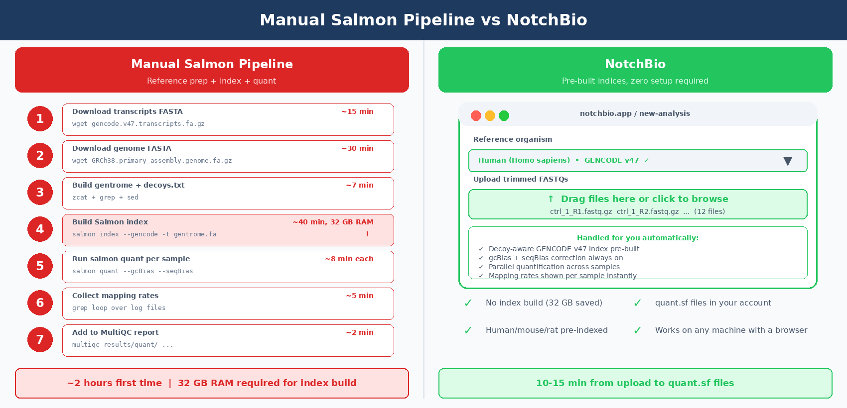
The Salmon pipeline above is solid and reproducible. But the reference download and index build alone take an hour before you can run a single sample.
Building the index requires 32 GB of RAM at peak. Most laptops cap out at 16 GB. You either need a workstation or HPC access just for the index build step.
NotchBio maintains pre-built, decoy-aware Salmon indices for human (GENCODE v47), mouse (GENCODE vM34), rat (Ensembl 110), and other common organisms. There is no index build step. You upload reads and select the organism.
| Step | Manual Salmon Pipeline | NotchBio |
|---|---|---|
| Reference download | ~45 min, manual URL lookup per organism | Not required |
| Build decoys.txt | 3 shell commands, grep + sed | Not required |
| Build gentrome | 5 min, zcat concat | Not required |
| Build Salmon index | 20-40 min, requires 32 GB RAM | Pre-built for human, mouse, rat, and more |
| Run salmon quant | 5-10 min per sample, bash loop | Parallel cloud execution |
| gcBias + seqBias | Flags you add manually | Always enabled |
| Collect mapping rates | grep loop across all log files | Shown in the dashboard per sample |
| MultiQC update | Re-run multiqc after quantification | Auto-updated in QC report |
| Index reuse | Yes, but only on same machine | Yes, across all uploads |
| RAM requirement | 32 GB for index build, 8 GB for quant | None — runs on our infrastructure |
| Time to first quant.sf | ~2 hours first time | 10-15 min from upload |
| Good for | Custom references, non-model organisms | Standard human/mouse/rat experiments |
If your organism is human, mouse, or rat and you want to skip the entire reference build, notchbio.app quantifies your reads with a pre-built decoy-aware GENCODE index. Upload your trimmed FASTQs and the quant.sf files are ready in minutes.
Further reading
Read another related post
The Reproducibility Crisis in Bulk RNA-Seq
Half of published RNA-seq pipelines fail when someone else tries to run them. A practitioner view of what breaks and how to build for reproducibility.
TutorialPyDESeq2 vs R DESeq2: Validation and the scanpy Workflow
Does PyDESeq2 really match R DESeq2? A tutorial on validating results against R, running PCA with scanpy and AnnData, and exporting DEGs for enrichment.
BioinformaticsWhy Reproducibility Should Not Be Optional in RNA-Seq Pipelines
Run snapshots, version pinning, and locked parameters should be the default, not a feature. A practitioner case for reproducibility-first RNA-seq platforms.