PyDESeq2 vs R DESeq2: Validation and the scanpy Workflow
Python users doing RNA-seq analysis have historically had two uncomfortable options: learn R well enough to run DESeq2, or use Python-native tools that do not implement the same statistical model. PyDESeq2 changes that. It is a faithful Python reimplementation of the DESeq2 negative binomial GLM, written by the Owkin team, and it integrates directly with AnnData objects and the scanpy ecosystem. If your analysis lives in Python and you want publication-grade differential expression without switching languages, PyDESeq2 is the current best option.
This tutorial leans into the two questions Python users actually worry about: can you trust that PyDESeq2 matches R, and how does it fit the scanpy ecosystem? We install the library, load count data, fit the model, extract results, validate them against an R DESeq2 baseline, run PCA with scanpy on the AnnData object, and export for enrichment analysis.
If you instead want the full feature reference, Differential Expression Analysis in Python with PyDESeq2: A Complete Tutorial is the comprehensive version, and From Salmon Output to DEGs in Python with PyDESeq2 covers building the count matrix straight from Salmon quant.sf files.
When To Choose PyDESeq2 Over R DESeq2
The choice is almost entirely about your existing ecosystem rather than statistical performance. The two implementations share the same mathematical model: negative binomial GLM with shrunken dispersion estimates and Wald tests. Results between them are close but not identical because they differ in some numerical details of the optimization routines.
Choose PyDESeq2 when your analysis pipeline is already Python-native, your count data lives in AnnData objects from a scanpy workflow, or you are building an automated analysis system in Python where calling out to R would complicate the architecture. Choose R DESeq2 when your team works primarily in R, when you are working with complex multi-factor designs where the R implementation has more battle-tested edge case handling, or when a reviewer specifically asks you to use R DESeq2 because it is the field standard.
The one situation where you should be cautious about PyDESeq2 is small sample sizes, below three replicates per group. In that regime the dispersion estimation can diverge slightly from the R implementation. In practice the difference is unlikely to change your conclusions, but it is worth validating against R if your sample sizes are small and the paper is high-stakes.
PyDESeq2 results are close but not identical to R DESeq2
PyDESeq2 implements the same statistical model as R DESeq2 but differs in some numerical details of the optimization. Expect log2 fold changes and adjusted p-values to be very similar but not exactly equal. For most experiments the differences are well below any meaningful threshold. For small sample sizes or complex designs, run a validation comparison against R DESeq2 before relying solely on PyDESeq2 results for publication.
Installation
# Install from PyPI# Requires Python 3.8 or laterpip install pydeseq2
# Optional but recommended: install anndata for AnnData input formatpip install anndata scanpy
# For plottingpip install seaborn matplotlib
PyDESeq2 has no R dependency. It is pure Python with numpy, scipy, and pandas under the hood.
Loading Count Data and Metadata
PyDESeq2 accepts count data as either a pandas DataFrame or an AnnData object. The DataFrame path is the simplest starting point if you are coming from a CSV count matrix.
import pandas as pdimport numpy as npfrom pydeseq2.dds import DeseqDataSetfrom pydeseq2.ds import DeseqStats
# Load the raw count matrix# Rows must be SAMPLES, columns must be GENES# This is the TRANSPOSE of the typical R conventioncounts_df = pd.read_csv("counts_matrix.csv", index_col=0)
# PyDESeq2 expects samples as rows, genes as columns# If your matrix has genes as rows, transpose itif counts_df.shape[0] > counts_df.shape[1]:    # Likely genes x samples, need to transpose    counts_df = counts_df.T
print(f"Shape: {counts_df.shape}")  # should be (n_samples, n_genes)
# Load sample metadatametadata_df = pd.read_csv("sample_metadata.csv", index_col=0)
# Ensure sample IDs match between counts and metadataassert all(counts_df.index == metadata_df.index), \    "Sample order mismatch between counts and metadata"
print(metadata_df)
The transposition is the most common point of confusion for people coming from R. DESeq2 in R expects genes as rows and samples as columns. PyDESeq2 follows the AnnData / scanpy convention where observations (samples) are rows and variables (genes) are columns. If you get this wrong, the model will appear to run but your results will be meaningless.
# Pre-filter: remove genes with fewer than 10 counts across all samples# PyDESeq2 does its own internal filtering but this speeds up computationgene_counts = counts_df.sum(axis=0)counts_filtered = counts_df.loc[:, gene_counts >= 10]
print(f"Genes after filtering: {counts_filtered.shape[1]}")
Building the DeseqDataSet and Fitting the Model
The DeseqDataSet object in PyDESeq2 is the equivalent of DESeqDataSet in R. It holds the count matrix, the metadata, and the design specification.
# Build the DeseqDataSet# design_factors: the column(s) in metadata to include in the modeldds = DeseqDataSet(    counts      = counts_filtered,    metadata    = metadata_df,    design_factors = "condition",   # equivalent to ~ condition in R    ref_level   = ["condition", "control"],  # set the reference level    n_cpus      = 4,                # parallel processing    refit_cooks = True              # refit for outlier samples (recommended))
# Run the full pipeline: size factor estimation, dispersion, GLM fitdds.deseq2()
The ref_level argument is important. It sets which condition is the denominator in your fold change calculation. Setting it explicitly prevents PyDESeq2 from defaulting to alphabetical order, which may give you the wrong direction of effect.
Extracting and Examining Results
After fitting the model, create a DeseqStats object to run the Wald test and extract results for a specific contrast.
# Run the Wald test for the contrast of intereststat_res = DeseqStats(    dds,    contrast   = ["condition", "treated", "control"],    alpha      = 0.05,    cooks_filter = True,    independent_filter = True)
# Run the test and apply Benjamini-Hochberg correctionstat_res.run_wald_test()stat_res.p_adjoust()   # applies BH correction
# Extract results as a DataFrameresults_df = stat_res.results_dfprint(results_df.head())print(f"\nTotal genes tested: {len(results_df)}")print(f"Significant (padj < 0.05): {(results_df['padj'] < 0.05).sum()}")
The results DataFrame has the same columns as the R DESeq2 output: baseMean, log2FoldChange, lfcSE, stat, pvalue, and padj. The column semantics are identical.
# Apply lfcShrink for better fold change estimates# PyDESeq2 implements the same apeglm-equivalent shrinkagestat_res.lfc_shrink(coeff="condition_treated_vs_control")
# Extract the filtered DEG tableresults_df = stat_res.results_df.copy()degs = results_df[    results_df["padj"].notna() &    (results_df["padj"] < 0.05) &    (results_df["log2FoldChange"].abs() >= 1)].copy()
print(f"DEGs up:   {(degs['log2FoldChange'] > 0).sum()}")print(f"DEGs down: {(degs['log2FoldChange'] < 0).sum()}")
Validation: Comparing Against R DESeq2
If your experiment is important enough to publish, it is worth spending 15 minutes running the same analysis in R and comparing the top results. The comparison does not need to be perfect; you are looking for major discrepancies, not numerical identity.
# Load R DESeq2 results (exported from R as a CSV)r_results = pd.read_csv("deseq2_r_results.csv", index_col=0)
# Merge on gene IDcomparison = results_df.join(    r_results[["log2FoldChange", "padj"]].rename(        columns={"log2FoldChange": "r_lfc", "padj": "r_padj"}    ),    how="inner")
# Correlation of log2FC estimateslfc_corr = comparison["log2FoldChange"].corr(comparison["r_lfc"])print(f"log2FC correlation (Python vs R): {lfc_corr:.4f}")# Expect > 0.99 for standard experiments
# Check that significant genes agreepython_sig = set(comparison[comparison["padj"] < 0.05].index)r_sig      = set(comparison[comparison["r_padj"] < 0.05].index)overlap    = len(python_sig & r_sig)print(f"Significant gene overlap: {overlap} / {len(python_sig | r_sig)}")
A log2FC correlation above 0.99 and a significant gene overlap above 95 percent means the two implementations agree well and you can proceed with the Python results. If either metric is substantially lower, investigate whether the reference levels, design formulas, and input matrices are truly equivalent between the two runs before proceeding.
PCA Plot with Scanpy
Visualizing sample separation before differential expression is a critical sanity check. If treated and control samples do not separate on the first two PCs, something is wrong with your data or metadata.
import scanpy as scimport anndata as ad
# Build an AnnData object from normalized counts for visualization# Use VST-transformed values or log1p of normalized counts# PyDESeq2 stores normalized counts in dds.layers["normed_counts"]adata = ad.AnnData(    X    = dds.layers["normed_counts"],    obs  = metadata_df,    var  = pd.DataFrame(index=counts_filtered.columns))
# Log-transform for PCAsc.pp.log1p(adata)
# Compute PCAsc.pp.pca(adata, n_comps=10)
# Plot colored by conditionsc.pl.pca(    adata,    color  = "condition",    title  = "PCA of normalized counts",    save   = "pca_condition.png")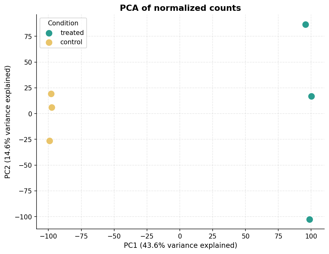
Volcano Plot with Matplotlib
import matplotlib.pyplot as pltimport matplotlib.patches as mpatchesimport numpy as np
# Prepare dataplot_df = results_df.copy()plot_df = plot_df[plot_df["padj"].notna()]plot_df["-log10padj"] = -np.log10(plot_df["padj"].clip(lower=1e-30))
# Assign colorsdef assign_color(row):    if row["padj"] < 0.05 and row["log2FoldChange"] >= 1:        return "up"    elif row["padj"] < 0.05 and row["log2FoldChange"] <= -1:        return "down"    return "ns"
plot_df["direction"] = plot_df.apply(assign_color, axis=1)
color_map = {"up": "#E63946", "down": "#457B9D", "ns": "#CCCCCC"}
fig, ax = plt.subplots(figsize=(8, 6))for direction, color in color_map.items():    subset = plot_df[plot_df["direction"] == direction]    ax.scatter(        subset["log2FoldChange"],        subset["-log10padj"],        c=color, s=15, alpha=0.6, linewidths=0, label=direction    )
# Threshold linesax.axhline(-np.log10(0.05), color="grey", linestyle="--", linewidth=0.8)ax.axvline(-1, color="grey", linestyle="--", linewidth=0.8)ax.axvline(1, color="grey", linestyle="--", linewidth=0.8)
ax.set_xlabel("Log2 fold change (treated vs control)", fontsize=12)ax.set_ylabel("-Log10 adjusted p-value", fontsize=12)ax.set_title("Differential expression: treated vs control", fontsize=13)ax.set_xlim(-6, 6)ax.set_ylim(0, 30)
up_count   = (plot_df["direction"] == "up").sum()down_count = (plot_df["direction"] == "down").sum()ax.legend(    handles=[        mpatches.Patch(color="#E63946", label=f"Up ({up_count})"),        mpatches.Patch(color="#457B9D", label=f"Down ({down_count})"),        mpatches.Patch(color="#CCCCCC", label="NS"),    ],    frameon=False)
plt.tight_layout()plt.savefig("volcano_treated_vs_control.png", dpi=300, bbox_inches="tight")plt.show()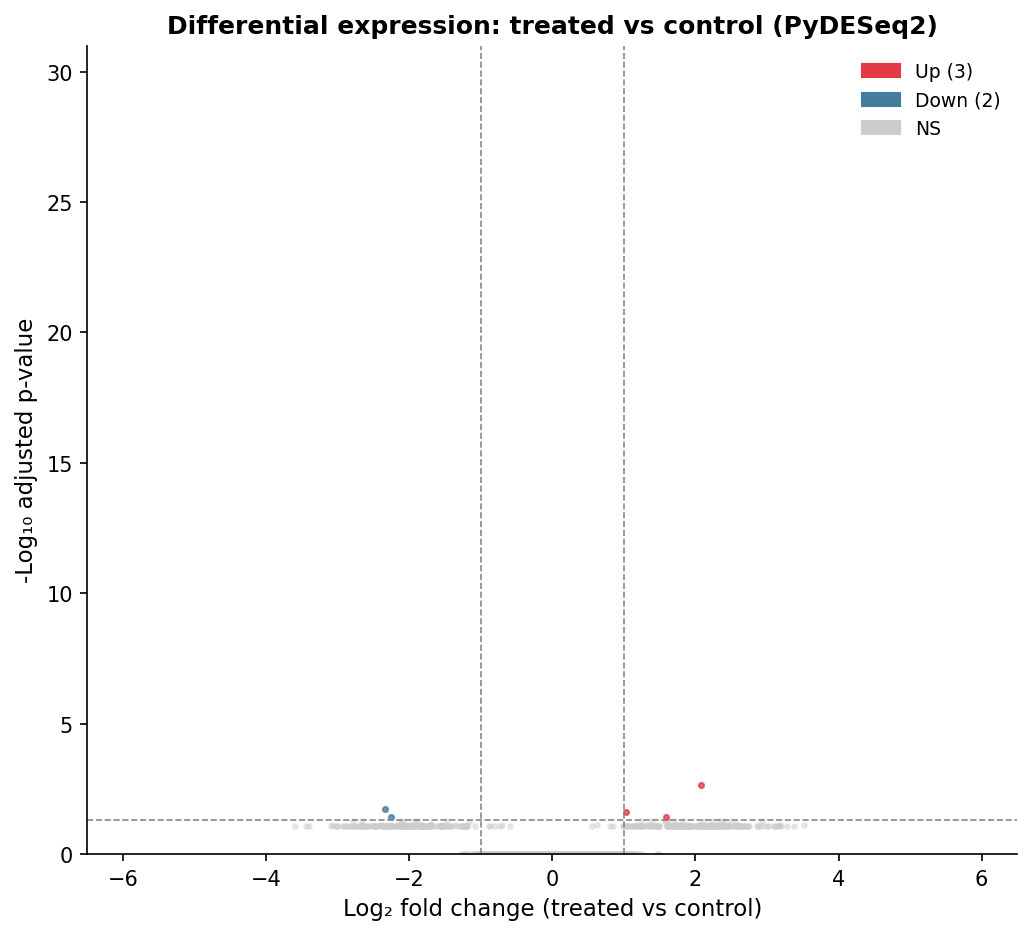
Exporting for Enrichment Analysis
The export format is the same as the R workflow: a full results table for GSEA input, and a filtered DEG list for ORA.
# Full results for GSEA (all tested genes, sorted by Wald stat)gsea_input = results_df[results_df["stat"].notna()].copy()gsea_input = gsea_input.sort_values("stat", ascending=False)gsea_input[["stat"]].to_csv("gsea_ranked_pydeseq2.csv")
# DEG list for ORAdegs.to_csv("degs_pydeseq2.csv")
# Background for ORA: all genes with non-null padjbackground = results_df[results_df["padj"].notna()].index.tolist()pd.Series(background).to_csv("ora_background.csv", index=False, header=False)
print(f"Exported {len(gsea_input)} genes for GSEA ranking")print(f"Exported {len(degs)} DEGs for ORA")print(f"Background size for ORA: {len(background)}")
Python vs R DE Library Comparison
| Library | Language | Implements DESeq2 model | AnnData support | Active maintenance | Best for |
|---|---|---|---|---|---|
| PyDESeq2 | Python | Yes (reimplementation) | Yes | Yes | Python-native pipelines, scanpy workflows |
| diffxpy | Python | No (Wald test on GLM) | Yes | Limited | Quick DE in scanpy, not publication-primary |
| edgeR via rpy2 | Python via R | Yes (edgeR) | Partial | Via rpy2 bridge | R-quality results from Python with complexity |
| DESeq2 via rpy2 | Python via R | Yes (original) | Partial | Via rpy2 bridge | Maximum fidelity to R DESeq2, harder to set up |
| pydeseq2 + pyGSEA | Python | Yes + enrichment | Yes | Yes | End-to-end Python DE and enrichment |
PyDESeq2 is the right choice for most Python-native workflows. If you need absolute fidelity to the original R implementation and are comfortable with the rpy2 bridge, the R-via-Python approach works but adds significant setup complexity.
NotchBio accepts a count matrix upload and returns results in both R-compatible and Python-compatible formats, including a pandas DataFrame export of the full results table and a ranked gene list ready for pyGSEA or gseapy. If you want the statistical rigor of DESeq2 without the language choice overhead, that is what the platform is built for.
Related Reading
Further reading
Read another related post
How to Run FastQC and MultiQC on Raw RNA-Seq Reads
A hands-on guide to automating RNA-seq QC across dozens of samples using FastQC and MultiQC, with bash and Python scripts for parsing and flagging failures.
Research GuideRaw Reads to Counts: The Bulk RNA-Seq Pipeline Explained
Every computational step in bulk RNA-seq, explained: from FASTQ quality control through trimming, alignment, and quantification to your final count matrix.
Research GuideWhat Are Batch Effects in RNA-Seq (and Why They Ruin Results)
What batch effects are, why they happen in bulk RNA-seq, and how they quietly corrupt your differential expression results — the concepts to grasp first.