Raw Reads to Counts: The Bulk RNA-Seq Pipeline Explained
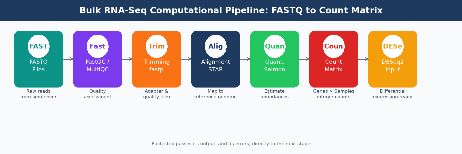
Your sequencing facility emails you a link to a folder of .fastq.gz files. Each file is a compressed archive of tens of millions of short DNA sequences, each paired with a quality score. It looks like noise. Getting from that to a count matrix you can hand to DESeq2 requires six distinct computational steps, and getting any one of them wrong can quietly corrupt every result downstream.
This post walks through the full computational pipeline, step by step: what each tool does, why it matters, what settings actually need your attention, and where the silent failures hide. The goal is not to replace documentation. It is to give you the mental model you need to understand what you are running and catch problems before they reach your gene lists. If you want the wet-lab context before FASTQ files even exist, read What Actually Happens to Your RNA Sample Before It Becomes Data. If you want the endpoint of this pipeline in more detail, read What Is a Count Matrix and Why Does It Matter.
Step 1: Initial Quality Control with FastQC and MultiQC
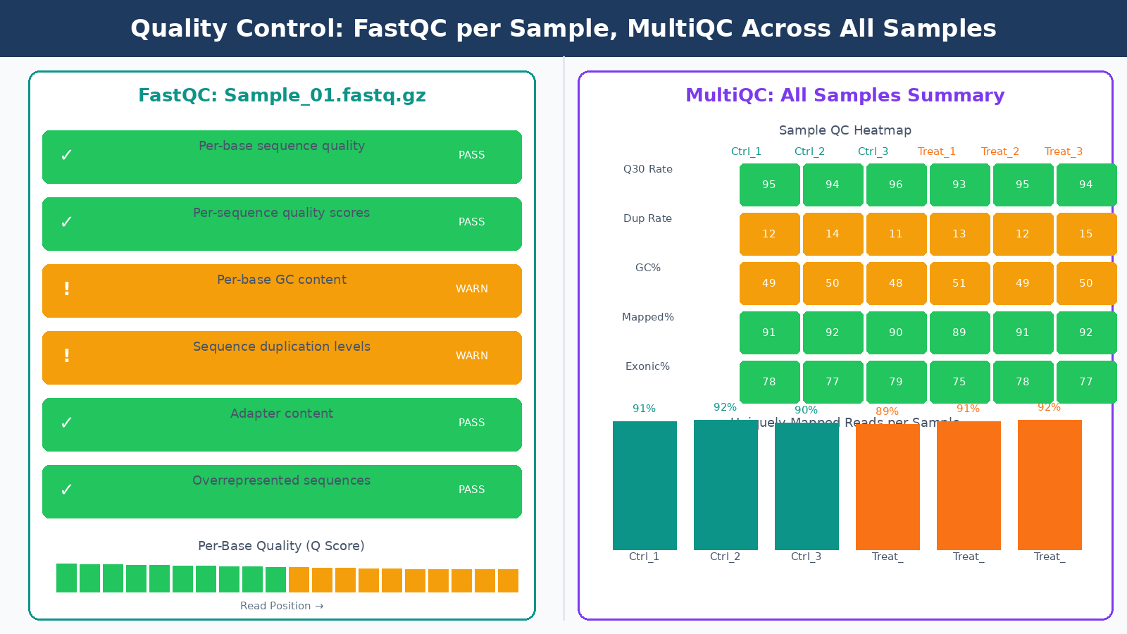
Before running any analysis, you need to know what your data actually looks like. FastQC generates a per-sample HTML report covering per-base quality scores, GC content, sequence duplication levels, adapter content, and k-mer enrichment. Each module gets a pass, warning, or fail flag. We cover that workflow in detail in How to Run FastQC and MultiQC on Raw RNA-Seq Reads.
Here is something worth knowing upfront: FastQC’s flag thresholds are specifically tuned for whole-genome shotgun DNA sequencing, which means they are less reliable for other types including RNA-seq. A “fail” on the per-sequence GC content module is expected for RNA-seq data because you are not sampling evenly from a genome; you are sampling from expressed transcripts with their own GC distribution. A “fail” on per-base sequence content in the first 10 to 12 bases is also normal, caused by random hexamer priming bias during library preparation. Do not let these flags send you into a panic spiral.
What you actually need to watch in FastQC for RNA-seq:
Per-base quality scores should stay above Q30 across most of the read length. Quality typically drops at the 3-prime end. A sequencing quality score of 30 or above is generally considered very good. If quality degrades sharply before the last 10 bases, trimming will help. If quality is poor from the start, the problem is with the run itself and no trimming will fix it.
Adapter content is the flag that matters most for deciding whether to trim. If you see adapter sequences climbing above a few percent of reads, trim them. If adapter content is near zero, trimming is optional.
Duplication rates in RNA-seq are not a quality failure. Highly expressed genes produce many identical reads by design. Do not remove duplicates from RNA-seq data the way you would for ChIP-seq or whole-genome sequencing.
Running FastQC on dozens of samples manually and comparing reports is tedious. MultiQC aggregates results from many bioinformatics tools, standardizing outputs and exporting data as TSV, YAML, or JSON alongside an HTML report. Run it once, get one report, compare all samples at a glance. It integrates with FastQC, STAR, Salmon, and most other tools in the pipeline. Any sample that looks like an outlier in the MultiQC heatmaps deserves a closer look before you proceed.
Outlier samples in MultiQC deserve investigation, not automatic removal
A sample with 40% lower mapping rate than its replicates, or a dramatically different GC content, might indicate a wet lab failure, a swap, or contamination. Investigate before deciding whether to exclude it. Removing samples without documented justification is not QC; it is p-hacking.
Step 2: Adapter Trimming with fastp or Trimmomatic
Trimming removes adapter sequences and low-quality bases from the ends of reads. The most commonly used tools are Trimmomatic and fastp. In practice, fastp has become the default in most modern pipelines. It is faster, handles paired-end reads more gracefully, and produces its own QC report alongside the trimmed output, so you do not need a separate FastQC run afterward.
The parameters that actually matter:
Minimum read length after trimming should be set to 25 to 35 bases. Reads shorter than this tend to align to many locations and produce noise in your count matrix. The exact cutoff depends on your read length; for 100bp reads, a 25bp floor is conservative enough.
Quality trimming uses a sliding window approach in Trimmomatic, or a per-base quality threshold in fastp. Aggressive trimming can improve alignment rates but can also introduce length bias. If your raw data quality is already good (most modern Illumina runs are), skip aggressive quality trimming and only remove adapters.
Do not trim if you do not need to. Some pipelines run trimming by default as a cargo-cult step. If your FastQC output shows no adapter contamination and good base quality, trimming adds processing time without improving results. Check first, trim if needed.
Step 3: Alignment or Pseudo-Alignment
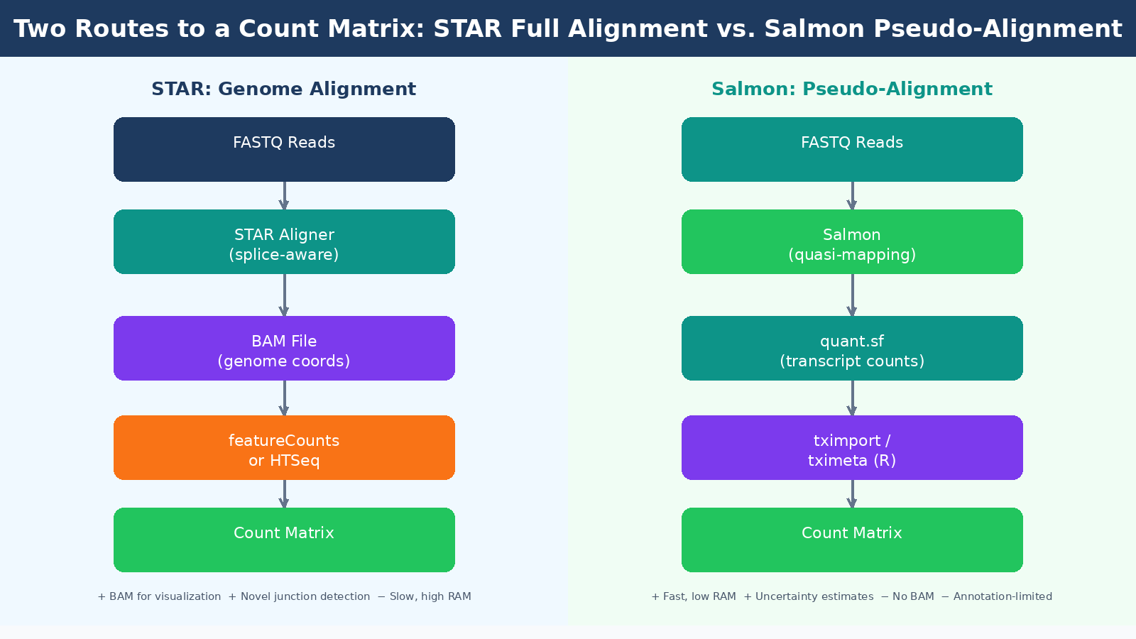
This is where the field has split into two camps, and you need to understand both.
Genome alignment with STAR maps your reads directly to a reference genome, producing a BAM file that records the exact genomic position of each read. STAR handles spliced alignment, which means it correctly maps reads that span exon-exon junctions. STAR achieves the lowest pseudo-false-positive rate in splice junction detection while also achieving the second highest sensitivity among tested aligners. The BAM files it produces can be loaded into a genome browser like IGV, which is useful for sanity-checking results, visualizing coverage patterns, and diagnosing alignment problems manually.
The cost of full alignment is computational. STAR requires about 30GB of RAM to build a human genome index and alignment takes longer than pseudo-alignment. For a 30-sample experiment on a well-provisioned server this is not a bottleneck, but on a laptop or a constrained HPC queue it matters.
Pseudo-alignment with Salmon takes a fundamentally different approach. Rather than finding the precise genomic position of each read, Salmon determines which transcripts a read is compatible with, then uses a statistical model to estimate abundance. Salmon and Kallisto only map to the transcriptome rather than the genome, and their results are only as good as the transcript annotation that is input into them. They cannot quantify genes or splice-variants that are not in their annotation, and they cannot be used for finding new genes, transcripts, or splice forms.
What they can do, they do very efficiently. STAR and Salmon used together for alignment and quantification showed a high correlation with results from the much faster pseudo-aligner Salmon alone, reaching 95% correlation in human cell datasets. For straightforward differential expression analysis against a well-annotated organism, Salmon’s pseudo-alignment is fast, accurate, and produces the uncertainty estimates that modern tools like tximport and tximeta are designed to consume.
| Feature | STAR (Full Alignment) | Salmon (Pseudo-Alignment) |
|---|---|---|
| Output | BAM file + counts | Quantification files (quant.sf) |
| Speed | Slower | Much faster |
| RAM requirement | ~30GB for human | ~8GB for human |
| Novel splice junctions | Detects them | Cannot detect them |
| Browser visualization | Yes (via BAM) | No |
| Uncertainty estimates | No | Yes |
| Best for | Novel transcriptomics, diagnostics | Standard DE analysis |
A widely adopted pattern in current pipelines is to run STAR for alignment and then use Salmon in alignment-based mode to quantify from the STAR BAM file. This gives you the visualization capability of a BAM file alongside Salmon’s probabilistic quantification. The nf-core/rnaseq pipeline implements this approach as its default green route, and it is a reasonable choice for most experiments.
Match your annotation version to your aligner index
If you build a STAR index using Ensembl GRCh38 release 110, your Salmon transcriptome index must come from the same release. Mismatching annotation versions between alignment and quantification steps creates subtle, hard-to-diagnose discrepancies in your count matrix that will not surface as obvious errors.
Step 4: Quantification and the Count Matrix
After alignment or pseudo-alignment, you need to aggregate reads into a count per gene per sample. How you get there depends on your approach.
If you used STAR, the most common quantification tools are featureCounts (from the Subread package), HTSeq-count, and RSEM. Each reads the BAM file and counts how many reads fall within annotated gene boundaries. The main parameter to configure is how to handle reads that overlap multiple genes. Multi-mapping reads are a genuine problem: a read from a gene family member may align equally well to two related genes, and how the tool assigns it affects your counts. Most tools discard ambiguous reads by default.
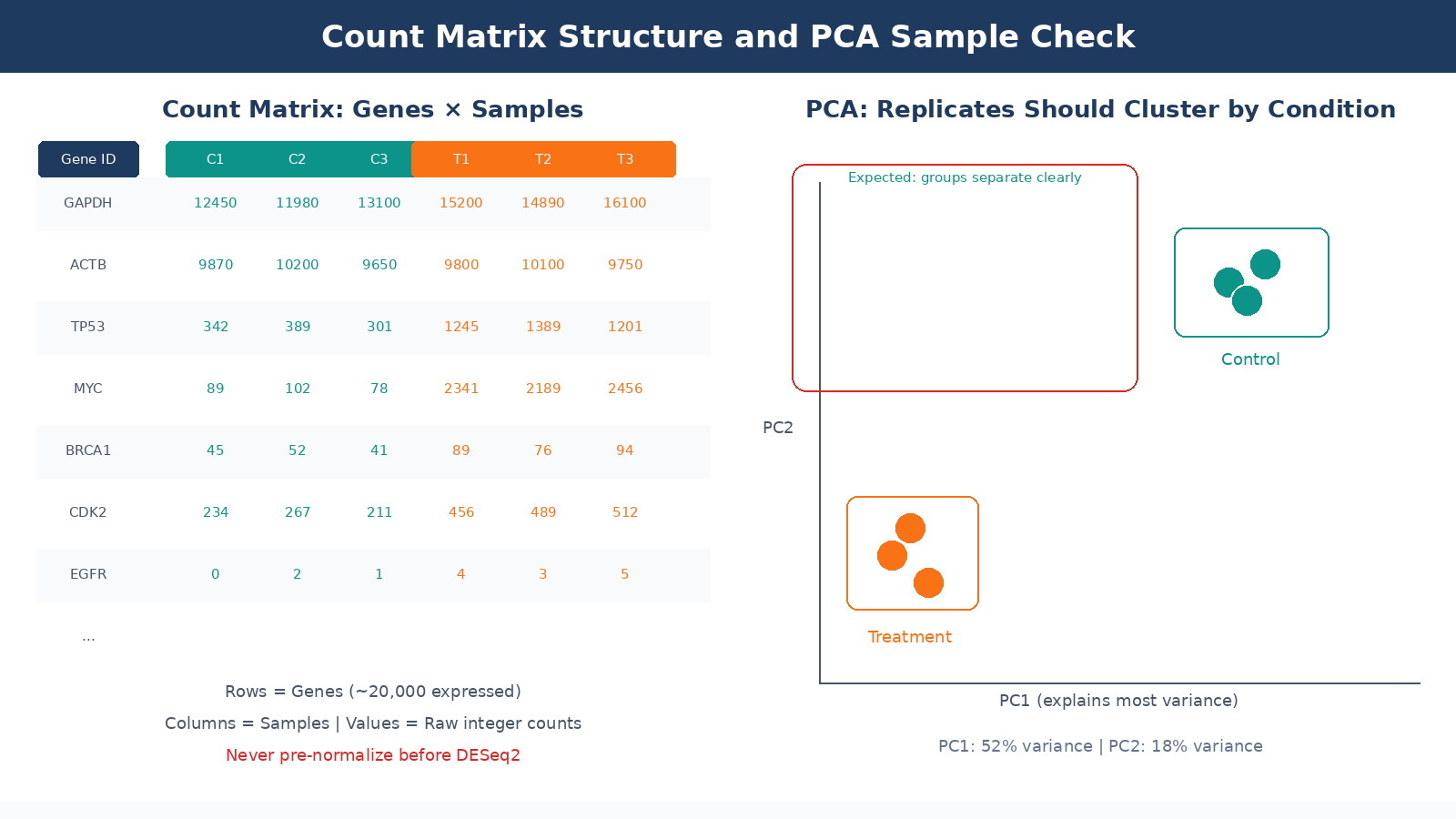
If you used Salmon, the output is a quant.sf file per sample containing transcript-level abundance estimates. These are not count matrices yet. You bring them into R using tximport or tximeta, which aggregates transcript-level estimates to the gene level and prepares the input for DESeq2. The values in the count matrix must be counts or estimated counts of sequencing reads or fragments. It is important to never provide counts that were pre-normalized for sequencing depth or library size, as the statistical model is most powerful when applied to un-normalized counts and is designed to account for library size differences internally.
This is a rule that gets broken surprisingly often. Researchers sometimes normalize their counts to TPM or RPKM before passing them to DESeq2, either because they read an old tutorial or because the numbers “look cleaner.” This is wrong. DESeq2 implements its own normalization through size factors calculated from raw counts. Pre-normalizing breaks this model.
Step 5: Post-Alignment QC
Getting a BAM file and a count matrix does not mean you are done with QC. Post-alignment metrics tell you things pre-alignment QC cannot.
Mapping rate is the percentage of reads that successfully aligned to the reference. For a well-prepared human or mouse RNA-seq sample with a clean library, you should expect 85 to 95 percent uniquely mapping reads with STAR. A mapping rate below 70 percent is a warning sign. It could indicate species contamination, poor library quality, a wrong reference genome, or a wrong strandedness parameter.
Strandedness is a parameter you must get right. Most modern library preparation protocols are strand-specific, meaning the sequencer reads in a defined orientation relative to the original RNA strand. If you run an aligner with the wrong strandedness setting, roughly half your reads get assigned antisense labels and your counts become meaningless. The 5-prime to 3-prime bias column in MultiQC output denotes whether data has 5-prime or 3-prime biases, and values approaching 0.5 or 2 warrant further investigation. If you do not know your library’s strandedness, tools like RSeQC infer_experiment.py can determine it from a BAM file before you commit to alignment parameters.
Exonic read proportion tells you how efficiently your sequencing captured mRNA. In a good poly-A selected library, you want 70 to 80 percent of reads mapping to exons. A high proportion of intronic reads suggests either ribo-depleted data (which captures pre-mRNA), DNA contamination, or a wrong annotation.
| Post-Alignment Metric | Expected Range | Concern If |
|---|---|---|
| Uniquely mapping rate (STAR) | 85 to 95% | Below 70% |
| Multi-mapping rate | Below 10% | Above 20% |
| Exonic reads (poly-A library) | 70 to 85% | Below 60% |
| Intronic reads | 10 to 20% | Above 40% |
| 5-prime to 3-prime bias | 0.9 to 1.1 | Below 0.5 or above 2.0 |
Step 6: Building and Inspecting the Count Matrix
The final count matrix is a table with genes as rows and samples as columns. Each cell is an integer: the number of reads assigned to that gene in that sample. This is the input to DESeq2.
Before you hand it off to your differential expression analysis, check it. Specifically:
Library size variation across samples should not be extreme. If one sample has 40 million reads and another has 8 million, that disparity will be handled by DESeq2’s size factor normalization, but very low-count samples may have poor sensitivity for lowly expressed genes. Flag samples with less than 10 million reads.
Low-count genes dominate the row count of most matrices. The human genome has around 60,000 annotated features, but only 15,000 to 20,000 will be expressed at detectable levels in a given cell type. Pre-filtering genes with fewer than 10 counts across all samples is standard practice. Pre-filtering the count matrix reduces the memory size requirements of the analysis and increases the speed of transformations and testing, though DESeq2 does also perform its own internal filtering automatically.
Sample-to-sample correlation is the most important sanity check. Biological replicates should correlate highly with each other and distinctly from samples of a different condition. Run a PCA or hierarchical clustering on variance-stabilized counts before you touch DE analysis. If your replicates cluster by prep date rather than condition, you have a batch effect problem to address before proceeding.
The count matrix is not the finish line
Differential expression analysis, normalization, and visualization all come after the count matrix. DESeq2, edgeR, and limma-voom each have their own statistical assumptions and appropriate use cases. Handing raw counts to the wrong model, or pre-normalizing before input, changes your results in ways that will not throw an error but will quietly affect which genes appear significant.
The Pipeline as a System
Every step described here propagates its outputs, and its errors, into every step that follows. A bad trimming decision inflates alignment runtime. A wrong strandedness parameter corrupts your count matrix silently. A pre-normalized input to DESeq2 breaks the statistical model without producing a warning message.
The practical lesson is to run MultiQC across the full pipeline, not just on the raw FASTQ files. Collect FastQC metrics, STAR alignment logs, Salmon quantification summaries, and post-alignment metrics into a single report. Inspect it before running DE analysis. Most problems that look like biology at the DESeq2 stage turn out to be technical artifacts that were visible earlier in the QC chain, but nobody looked.
If you want to run this pipeline without building it from scratch, NotchBio automates the full FASTQ-to-count-matrix workflow with built-in QC checkpoints at each stage. You get the MultiQC report, alignment statistics, and a DESeq2-ready count matrix without configuring each tool individually. For labs running RNA-seq regularly, that means less time debugging shell scripts and more time interpreting results.
Further reading
Read another related post
How to Build a Salmon Index and Quantify Bulk RNA-Seq Reads
Step-by-step Salmon tutorial: download GENCODE references, build a decoy-aware index, run salmon quant with gcBias and seqBias on all samples, and verify mapping rates before DESeq2.
TutorialHow to Run FASTQ Quality Control with FastQC, fastp, and MultiQC
Full pipeline tutorial for bulk RNA-seq QC: run FastQC on raw reads, trim adapters with fastp, rerun QC, and aggregate reports with MultiQC. Includes parallel processing and how to read results.
TutorialHow to Download RNA-Seq Data from GEO and SRA Using sra-tools and pysradb
Step-by-step tutorial for downloading bulk RNA-seq FASTQ files from GEO and SRA. Covers prefetch, fasterq-dump, pysradb metadata extraction, batch downloads, and fixes for common errors.