What Actually Happens to Your RNA Sample Before It Becomes Data
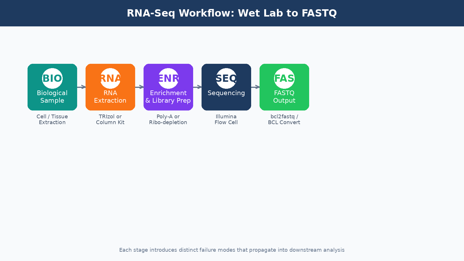
Most researchers treat the FASTQ file as the starting line. It is not. By the time your data lands on a compute cluster, your RNA has already survived extraction, survived fragmentation, been reverse-transcribed, amplified, size-selected, and shot through a flow cell at millions of reads per second. Everything that goes wrong before that point is invisible in the file, but it shapes every downstream result you will ever produce from that experiment.
This post walks through the full pre-computational journey of a bulk RNA-seq sample: from the moment you lyse your cells to the moment a FASTQ file appears in your project directory. Understanding this process will not just make you a better analyst. It will make you a better experimentalist, and it will help you diagnose failures that no bioinformatics tool can fix after the fact. Once the FASTQ files exist, the next stop is Raw Reads to Counts: The Bulk RNA-Seq Pipeline Explained, followed by How to Run FastQC and MultiQC on Raw RNA-Seq Reads for your first computational QC pass.
RNA Extraction: Where Most Experiments Are Won or Lost
The goal of extraction is simple: isolate intact, high-quality total RNA from your biological material. The reality is messier.
RNA is inherently unstable. RNases are everywhere: on your bench, in your reagents, on your hands. A few seconds of careless handling between tissue dissection and lysis buffer can degrade your sample enough to skew expression results toward highly stable transcripts and away from labile ones. This is not a hypothetical. Studies comparing RNA integrity scores across labs processing the same tissue type routinely show significant variance.
The two most common extraction approaches are column-based kits (like Qiagen RNeasy) and TRIzol-based phenol-chloroform extraction. Column kits are faster and more reproducible across users. TRIzol recoveries can be higher for certain tissues, especially those rich in lipids or polysaccharides, but the protocol demands more care. For most standard cell line or tissue experiments, a column-based kit with the optional on-column DNase digestion step is the right call.
Always run a DNase digestion step
Genomic DNA contamination is common and easy to miss. It will co-purify with your RNA and inflate your quantification numbers. On-column or in-solution DNase treatment before library prep is not optional if you care about your results.
After extraction, you need to assess quality before you do anything else. The two metrics that matter most are:
RNA Integrity Number (RIN), measured by a Bioanalyzer or TapeStation. RIN scores run from 1 (completely degraded) to 10 (perfectly intact). For most bulk RNA-seq applications, you want a RIN above 7. Samples below 6 should not proceed to library prep without serious justification.
260/280 absorbance ratio, measured by a NanoDrop. A ratio around 2.0 indicates pure RNA. Values significantly below 1.8 suggest protein contamination. Values above 2.1 can indicate phenol carryover from TRIzol extractions.
| Quality Metric | Acceptable Range | Concern Threshold | Likely Cause if Failed |
|---|---|---|---|
| RIN Score | 7.0 to 10.0 | Below 6.0 | Degradation during extraction or storage |
| 260/280 Ratio | 1.9 to 2.1 | Below 1.8 | Protein or phenol contamination |
| 260/230 Ratio | 2.0 to 2.2 | Below 1.5 | Guanidinium or ethanol carryover |
| Concentration | Kit-dependent | Below 10 ng/µL | Low input material or extraction failure |
Poly-A Selection vs. Ribosomal Depletion: Choosing Your Enrichment Strategy
Total RNA extracted from a eukaryotic cell is roughly 80 to 85 percent ribosomal RNA. rRNA carries no useful information for gene expression analysis, so it has to go. There are two main strategies for removing it.
Poly-A selection uses oligo-dT beads to capture messenger RNAs by their polyadenylated tails. It is efficient, cost-effective, and produces clean libraries with a high proportion of exonic reads. The problem is that it requires moderately intact RNA. Degraded RNA loses its poly-A tail first, so if your RIN is below 7, you will systematically lose reads from the 5-prime ends of transcripts and introduce length bias into your quantification.
Ribosomal RNA depletion (ribo-depletion) removes rRNA using hybridization probes rather than selecting for mRNA directly. It works on degraded samples and captures non-polyadenylated transcripts, including many lncRNAs. The tradeoff is cost, about two to three times more expensive per sample, and it requires species-specific probe sets that need to match your organism accurately.
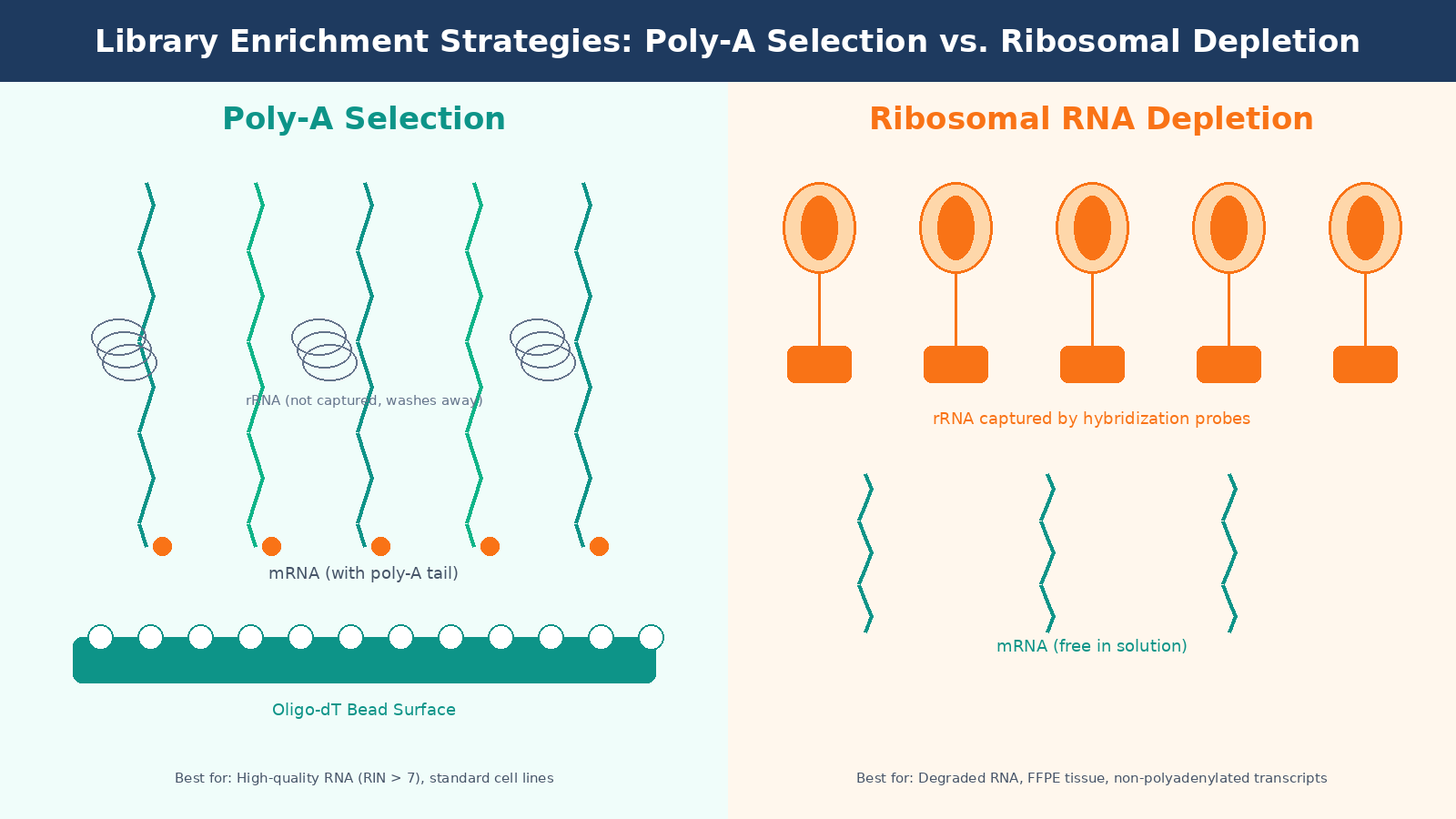
For standard cell line experiments with good RNA quality, poly-A selection is the default. For clinical samples, FFPE tissue, or any situation where RNA integrity is compromised, ribo-depletion is the more honest choice even if it costs more.
Library Preparation: Fragmentation, Reverse Transcription, and Adapter Ligation
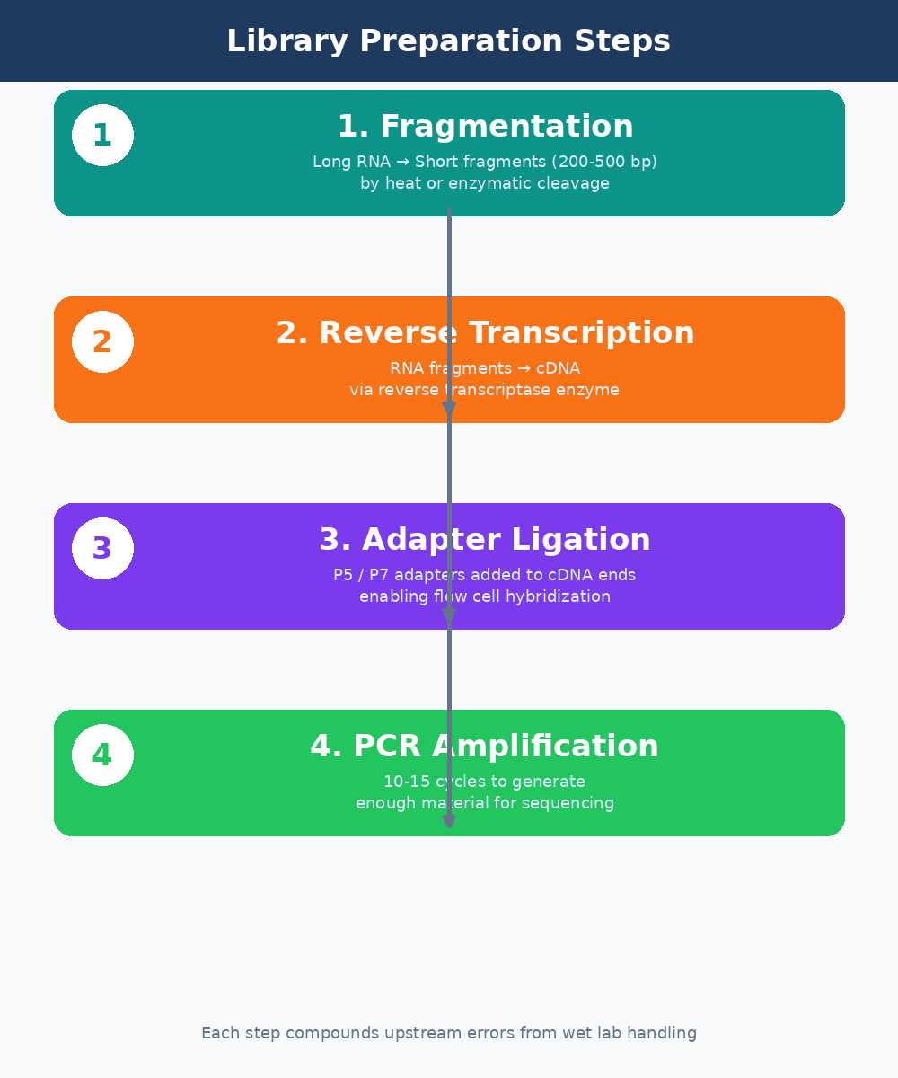
Once you have enriched for the RNA fraction you care about, library prep converts those RNA molecules into double-stranded cDNA fragments that can be loaded onto a sequencer. This process has several steps, each with failure modes that propagate invisibly into your data.
Fragmentation breaks RNA into pieces of 200 to 500 base pairs. Most modern kits use chemical fragmentation at elevated temperature. The fragmentation time matters. Under-fragmentation produces long inserts that sequence poorly. Over-fragmentation degrades your library and increases the proportion of adapter dimers. The optimal time varies with RNA concentration and integrity, and most protocol optimizations fail here.
Reverse transcription converts the fragmented RNA to cDNA using a reverse transcriptase enzyme. This step introduces its own biases. GC-rich sequences are converted less efficiently than AT-rich ones. Secondary structures in the RNA template can stall the enzyme. These biases are real and measurable, and they contribute to the variance you see in lowly-expressed transcript quantification.
Adapter ligation attaches short DNA sequences (adapters) to both ends of each cDNA fragment. These adapters serve two purposes: they allow the fragments to hybridize to the flow cell surface, and they contain the index sequences used to demultiplex multiplexed samples. Ligation efficiency is a common failure point. Low ligation efficiency produces libraries with high adapter dimer content, which wastes sequencing capacity and shows up clearly in FastQC output.
Strand specificity matters for library interpretation
Most modern bulk RNA-seq protocols are strand-specific (dUTP method or equivalent). Make sure you know whether your library is stranded and in which orientation before you run your alignment. Passing an unstranded library to a stranded aligner, or vice versa, can silently misassign up to 50 percent of your reads.
PCR Amplification and Size Selection
After ligation, the library is PCR amplified to generate enough material for sequencing. This is where duplicate reads are introduced. PCR duplicates are identical sequence reads that originate from the same original RNA molecule rather than from distinct transcripts. High duplication rates can compress your dynamic range and make lowly-expressed genes harder to detect.
The number of PCR cycles matters. Most protocols recommend 10 to 15 cycles for standard inputs. More cycles increase duplicates. Fewer cycles work only with high-input libraries. If you are working with limiting material (bulk RNA from sorted cell populations, for example), you need a low-input protocol optimized to minimize PCR jackpotting.
Size selection, either by gel extraction or SPRI bead-based cleanup, removes adapter dimers and size-outlier fragments from the final library. A library that skips size selection or performs it carelessly will have a broad insert size distribution that complicates downstream analysis and wastes reads on uninformative adapter sequences.
Sequencing on the Flow Cell: What the Machine Is Actually Doing
The final prepared library is loaded onto a sequencing flow cell. In Illumina sequencing, which dominates bulk RNA-seq, the flow cell surface is covered in oligonucleotides complementary to the adapter sequences on your library fragments. Each fragment hybridizes, is amplified locally into a cluster, and is then sequenced by synthesis: one fluorescently-labeled nucleotide at a time, photographed after each incorporation.
Read length and sequencing depth are the two parameters you configure when placing your sequencing order. For differential expression analysis of a standard transcriptome, 75 to 100 base pair paired-end reads at 20 to 30 million reads per sample is the commonly accepted minimum. For rarer transcripts, isoform analysis, or organisms with poorly annotated genomes, you need more depth.
The output of the sequencer is a FASTQ file: a text file where each read is represented by four lines. The sequence itself, the quality scores encoded as ASCII characters, the read identifier, and a separator line. The quality scores tell you, per base, how confident the instrument is in each base call. This is what FastQC reads to generate its per-base quality plots.
Paired-end vs single-end sequencing
Paired-end sequencing reads both ends of each library fragment. It roughly doubles your data and significantly improves alignment accuracy, especially for reads that span splice junctions or land in repetitive regions. For most bulk RNA-seq applications, paired-end 100bp is the standard. Single-end is only worth considering when cost is the primary constraint and your research questions are simple.
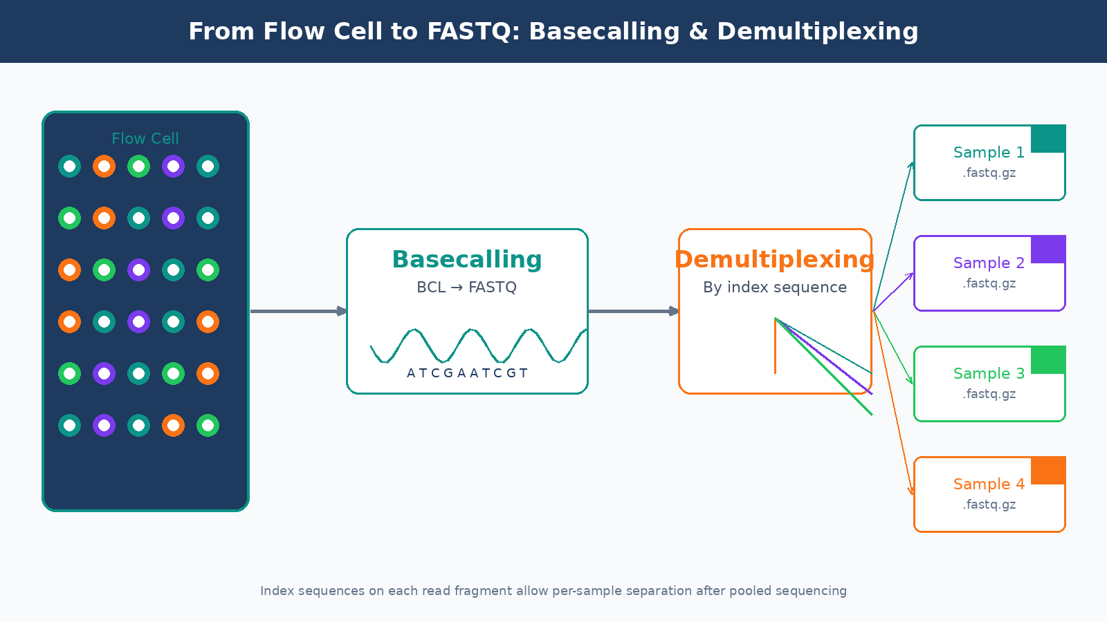
From Sequencer to FASTQ: Basecalling and Demultiplexing
The raw output of an Illumina instrument is not a FASTQ file. It is a proprietary binary format called BCL (Base Call files). The conversion from BCL to FASTQ happens through a process called basecalling, run by Illumina’s bcl2fastq or the newer BCL Convert tool. This step also handles demultiplexing: separating the reads from different samples based on their index sequences.
Index hopping is a known failure mode in demultiplexing, particularly on patterned flow cells (NovaSeq, NextSeq 2000). A small but non-trivial fraction of reads get assigned to the wrong sample index during the sequencing run. On standard runs this is usually below one percent, but it can be higher with poorly balanced index sets or when library concentrations vary widely across samples in a pool.
By the time you receive your FASTQ files from a core facility or commercial sequencing service, basecalling and demultiplexing are already done. But it is worth asking your sequencing provider what software version they used, what mismatch tolerance they allowed during demultiplexing, and whether they ran any initial QC on the run metrics. These details matter for diagnosing problems that show up later in your analysis.
What Can Go Wrong and How It Shows Up Downstream
Every step above introduces potential errors that arrive silently in your FASTQ files and propagate through your analysis. Here is a condensed map of the most common failure modes and where they surface:
| Wet Lab Failure | Where It Shows in Data |
|---|---|
| RNA degradation (low RIN) | 3-prime bias in coverage, low mapping rates, poor correlation between replicates |
| DNA contamination | Elevated reads mapping to introns, inflated gene counts |
| Adapter dimer contamination | High adapter content in FastQC, low insert size peak |
| Over-amplification (PCR) | High duplication rates, compressed dynamic range |
| Index hopping | Unexpected reads in negative controls, sample cross-contamination |
| Wrong strandedness specified | Reversed sense/antisense counts, apparent antisense expression |
| Batch effects from library prep | PC1 in PCA separates by prep date rather than condition |
This is the core argument for investing in your wet lab QC before you touch the compute side. A bioinformatics pipeline cannot rescue a degraded library. It cannot remove DNA contamination that looks like expressed genes. It cannot unscramble index-hopped reads. The data you feed into your pipeline is the ceiling on the quality of your results.
Running the Full Pipeline Without Starting from Scratch
Once you have clean FASTQ files, the computational pipeline begins: QC with FastQC and MultiQC, trimming with fastp or Trimmomatic, alignment or pseudo-alignment, and quantification into a count matrix. Each of those steps has its own configuration decisions and failure modes.
If you want to run a complete, reproducible bulk RNA-seq pipeline without building it from scratch, NotchBio automates the full workflow from FASTQ to differential expression results. You upload your files, specify your experimental design, and the platform handles QC, alignment, quantification, and DE analysis with auditable parameters. It is particularly useful for labs that run RNA-seq regularly but do not have dedicated bioinformatics staff to maintain a custom pipeline.
The goal of this post was not to turn you into a library prep expert overnight. It was to give you enough context that when something goes wrong in your analysis, you know which questions to ask before blaming the aligner. The FASTQ file is not the starting line. It is just where the computational work begins.
Further reading
Read another related post
GTF and GFF Files: Why They Hurt and How To Tame Them
GTF and GFF files from the same database often disagree, prokaryotic files lack exon features, AGAT fixes some and breaks others. A practical field guide.
BioinformaticsIndustrial Bioinformatics Is Still In Its Infancy
Most commercial bioinformatics runs on academic instincts. A senior practitioner view on what industry needs and the engineering practices that close the gap.
TutorialYour First Nextflow Pipeline for RNA-Seq (Without Losing Your Mind)
A minimal Nextflow DSL2 RNA-seq pipeline in under 80 lines: three processes, channel wiring, Docker config, and how to read the execution report and DAG output.