What Is a Count Matrix and Why Does It Matter
The count matrix is the central artifact of every bulk RNA-seq analysis. Everything upstream of it, the sequencing, the alignment, the quantification, exists to produce it. Everything downstream of it, the differential expression, the visualization, the pathway analysis, consumes it. And yet the count matrix is also one of the most commonly misused objects in bioinformatics.
The specific misuse is this: researchers normalize their counts for presentation or visualization purposes, and then feed those normalized values into a tool that expects raw counts. Or they use FPKM values to compare expression across samples, not realizing that FPKM comparisons across samples are mathematically invalid. Or they run DESeq2 on TPM values and wonder why the results look strange. None of these produce an error message. They all produce a number. The number is just wrong.
This post is about what the count matrix actually contains, what the various normalization schemes do and why they exist, and which form of expression data belongs in which downstream analysis. If you need to revisit where the matrix comes from, start with Raw Reads to Counts: The Bulk RNA-Seq Pipeline Explained. If your downstream interpretation is being distorted by design or technical artifacts, also read Experimental Design Mistakes That Kill Your Differential Expression Analysis and Batch Effects Will Ruin Your RNA-Seq Results.
What the Count Matrix Actually Contains
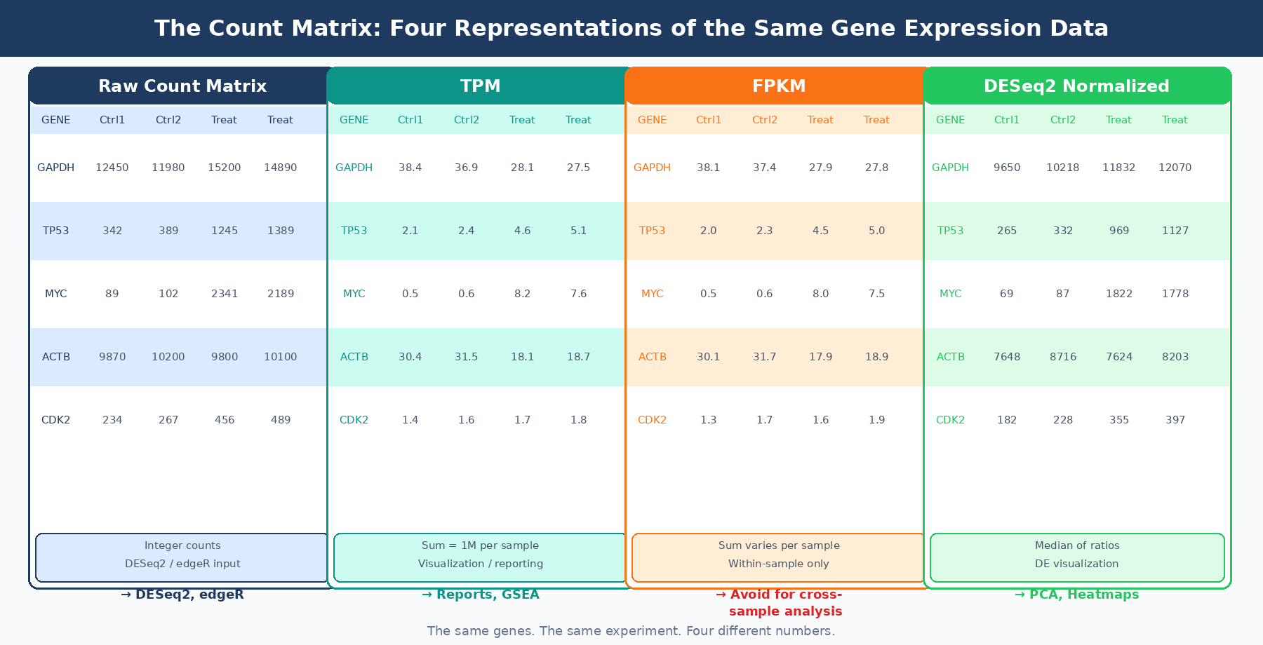
A count matrix is a rectangular table where each row is a gene and each column is a sample. Each cell contains an integer: the number of sequencing reads (or read pairs, for paired-end data) that were assigned to that gene in that sample.
These are not the number of RNA molecules. They are a proxy for expression, filtered through library preparation efficiency, sequencing depth, RNA extraction yield, gene length, and the annotation-dependent ambiguity of multi-mapping reads. A gene with 10,000 counts is not necessarily more expressed than a gene with 5,000 counts in the same sample, because the 10,000-count gene might simply be three times longer.
The raw count is also not comparable across samples unless the samples have identical library sizes, which they never do. A sample sequenced to 40 million reads will produce roughly twice the raw counts as the same sample sequenced to 20 million reads, for every gene, regardless of biology.
These two problems, incomparability within a sample due to gene length and incomparability across samples due to sequencing depth, are what the various normalization metrics attempt to solve. They solve them in different orders, with different assumptions, and with different downstream consequences.
RPKM and FPKM: The Legacy Metrics
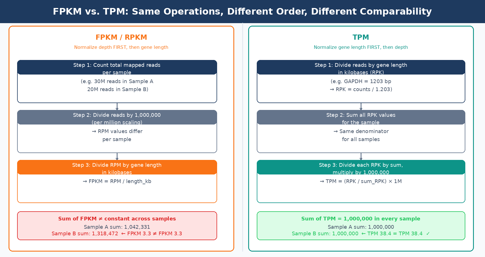
RPKM (Reads Per Kilobase per Million mapped reads) was introduced in 2008 by Mortazavi et al. to make gene expression values comparable both within and across samples in a single calculation. FPKM (Fragments Per Kilobase per Million) is the paired-end version of the same metric. The calculation normalizes first for library size (divides by total mapped reads in millions), then for gene length (divides by gene length in kilobases). The result is intended to be interpretable as a measure of relative RNA abundance that can be compared to any other gene in any other sample.
The problem is that FPKM does not actually achieve the cross-sample comparability it promises. When you normalize by total mapped reads, the denominator differs between samples. This means the sum of all FPKM values in sample A will be different from the sum in sample B. If those sums are different, then the FPKM value of 3.33 for gene X in sample A does not mean the same thing as an FPKM of 3.33 in sample B. You cannot directly compare them (RNA-Seq Blog, StatQuest).
The NCBI GEO documentation makes this explicit: FPKM and TPM counts should not be used for quantitative comparisons across samples when the total RNA contents and its distributions are very different. A common misconception is that RPKM and TPM values are already normalized, and thus should be comparable across samples or RNA-seq projects. However, RPKM and TPM represent the relative abundance of a transcript among a population of sequenced transcripts, and therefore depend on the composition of the RNA population in a sample (NCBI GEO).
Despite this, RPKM and FPKM remain embedded in many published datasets, older pipelines, and public repositories. If you receive FPKM values from a collaborator or a GEO download and need to do cross-sample analysis, convert them to TPM first. The conversion is straightforward: for each sample, divide each FPKM value by the sum of all FPKM values in that sample, then multiply by one million.
Never input FPKM or RPKM values into DESeq2 or edgeR
Both tools model the statistical distribution of raw integer counts. FPKM and RPKM values are continuous, fractional, and scaled differently per sample. Feeding them into DESeq2 will produce results, but those results are statistically invalid. The model’s negative binomial assumptions hold for raw counts, not for length-normalized ratios.
TPM: A Better Relative Abundance Metric
TPM (Transcripts Per Kilobase Million) solves the cross-sample comparability problem that FPKM gets wrong, by reversing the order of the two normalization steps.
For FPKM, the calculation is: divide by library size first, then divide by gene length. For TPM, the calculation is: divide by gene length first, then divide by the sum of all length-normalized values.
This seemingly small difference has a profound consequence: when you calculate TPM, the sum of all TPM values in every sample is exactly one million. This means TPM values represent the same thing in every sample: the fraction of length-adjusted expression attributable to that gene, scaled to a million. A TPM of 100 for gene X means the same proportion of your sequencing capacity was attributed to that gene regardless of which sample you are looking at (RNA-Seq Blog).
TPM is the right metric when you want to report relative expression levels for visualization, compare expression of different genes within a sample, or provide values for tools that work with expression proportions, like some GSEA rank-based methods. Salmon and kallisto both output TPM natively, which is one reason pseudo-alignment pipelines have largely moved away from FPKM.
But TPM has its own limitation for differential expression analysis. Like FPKM, it normalizes for gene length, and gene length is not a relevant factor when comparing the same gene across conditions. When you compare gene X in treated versus control samples, both gene X values have been divided by the same gene length. The length correction cancels out and adds no value. What it does do is change the statistical distribution of the counts from integer-valued to continuous and fractional, which breaks the negative binomial model that DESeq2 depends on.
DESeq2’s Median of Ratios: What Your DE Tool Actually Does
When you run DESeq2, it does not use TPM or FPKM. It takes your raw integer count matrix and performs its own normalization internally before fitting the statistical model. Understanding this normalization matters because it tells you why raw counts are the correct input and why pre-normalizing corrupts the analysis.
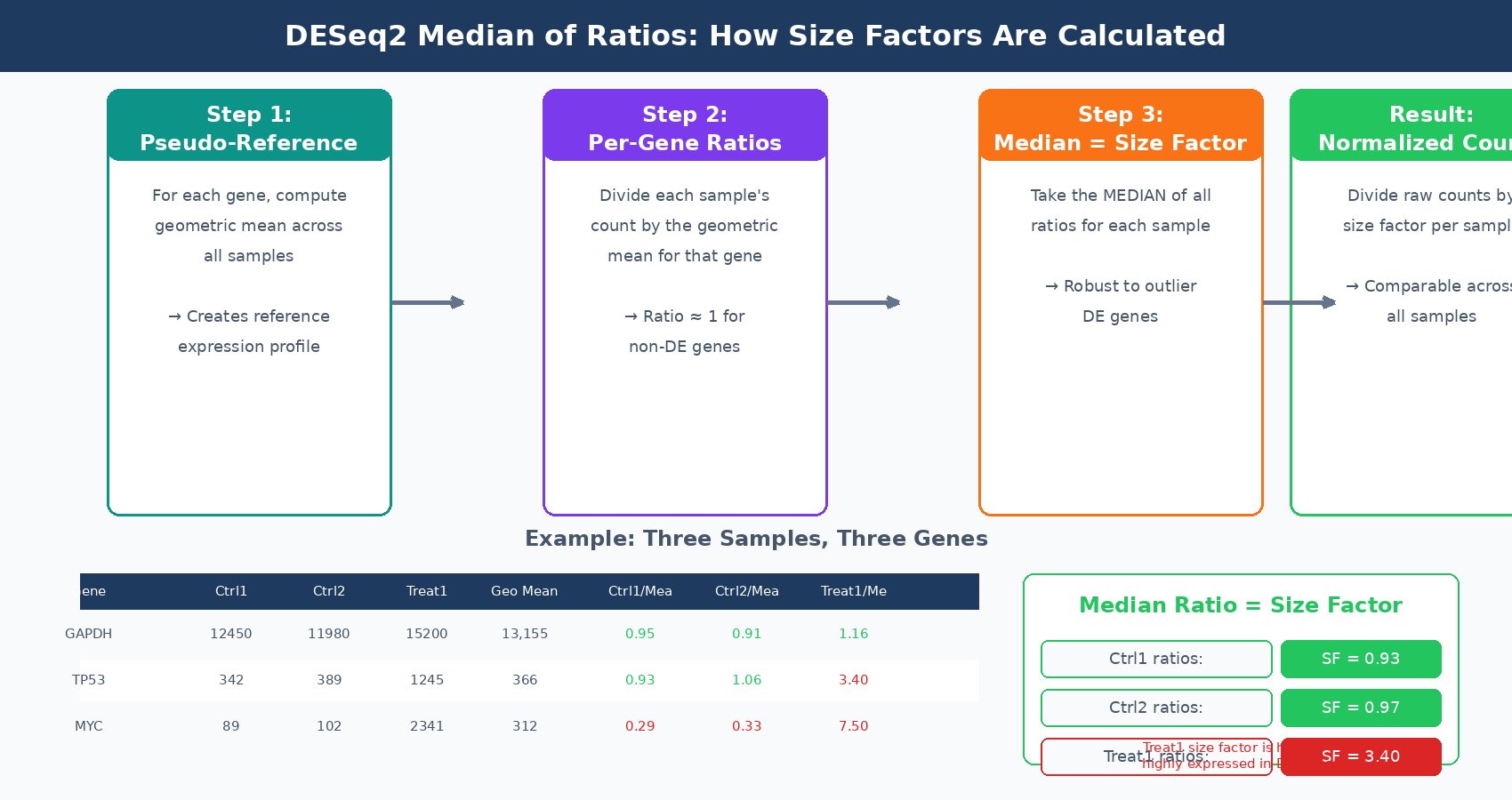
DESeq2 uses the median of ratios method (Harvard HBC Training). The procedure works in three steps:
First, for each gene, compute the geometric mean of its raw counts across all samples. This creates a pseudo-reference sample that represents the average expression profile of the experiment.
Second, for each sample, compute the ratio of each gene’s count to its geometric mean value across samples. These ratios capture how each sample’s library differs from the pseudo-reference.
Third, take the median of all these ratios for each sample. This median is the size factor. The median, rather than the mean, is used because it is robust to outliers. A handful of highly differentially expressed genes will appear in the tails of the ratio distribution, but the median ignores them. The size factor reflects the scaling factor needed to make the bulk of non-differentially expressed genes comparable across samples.
The key property of this approach is that it normalizes for both sequencing depth and RNA composition. RNA composition is the problem that simple library-size normalization misses: if a small number of genes are massively overexpressed in one condition but not another, dividing by total library size will make all other genes in that condition appear artificially underexpressed. The median of ratios method is resistant to this because those extreme genes are outliers in the ratio distribution and do not drive the median.
DESeq2 does not actually transform the raw counts before fitting the model. Rather, the size factors are incorporated as offsets in the generalized linear model itself. When DESeq2 says a gene is differentially expressed, it has already accounted for the size factors in its statistical test. The normalized count values you can extract with counts(dds, normalized=TRUE) are useful for visualization and quality control, but they are not what DESeq2 uses internally for the statistical test.
DESeq2 models normalization inside the GLM, not before it
A common misunderstanding is that DESeq2 first normalizes counts and then tests. It does not. DESeq2 uses raw counts as input and models the size factors as parameters within the negative binomial GLM. The normalized counts you extract afterward are a downstream product for human inspection, not the numbers the statistical test operated on.
VST and rlog: Normalization for Visualization and Clustering
DESeq2 produces two additional count transformations that are specifically designed for visualization and unsupervised analysis: variance stabilizing transformation (VST) and regularized log transformation (rlog).
Raw counts have a property called heteroscedasticity: their variance increases with their mean. A gene with a mean count of 10,000 will have much higher variance than a gene with a mean count of 100, even if the biological variability is similar. This makes it difficult to cluster samples or run PCA, because high-count genes will dominate the distance calculations regardless of whether they are biologically informative.
VST and rlog both solve this by transforming counts into a space where variance is approximately independent of the mean. VST is faster and preferred for large sample sizes (more than 30 samples). rlog is slower but better calibrated for small sample sizes. Neither output should be used as input to differential expression tests. They are for PCA, sample clustering, heatmaps, and other visualizations where you want all genes to contribute proportionally to the distance metric.
The practical rule is: use raw counts for DESeq2 input; use VST or rlog counts for PCA, clustering, and heatmaps; use TPM for within-experiment visualization and for reporting relative expression levels; do not use FPKM or RPKM for anything involving cross-sample comparison.
The Downstream Decision Table
| Task | Correct Input | Why |
|---|---|---|
| Differential expression (DESeq2) | Raw integer counts | Median of ratios normalization happens inside the GLM |
| Differential expression (edgeR) | Raw integer counts | TMM normalization is applied internally |
| PCA and sample clustering | VST or rlog counts | Variance-stabilized for equal contribution across expression range |
| Gene expression heatmap | VST or rlog, or TPM | Stabilized variance for interpretable color scaling |
| Within-sample gene ranking | TPM | Same gene length normalization applied to all genes in sample |
| Cross-sample expression comparison (reporting) | TPM | Sum of all TPMs is equal across samples |
| Cross-sample expression comparison (formal) | DESeq2 normalized counts | Accounts for RNA composition bias, not just depth |
| GSEA pre-ranked input | TPM or log2FC from DESeq2 | Rank-based; absolute values matter less than ordering |
| Cross-study meta-analysis | DESeq2 or TMM normalized | Controls for library composition across different experiments |
| Sharing with collaborators (GEO) | Raw counts + TPM | Raw counts for analysis; TPM for easy inspection |
The Most Dangerous Mistake: Feeding Normalized Counts to DESeq2
In my experience, the most damaging count matrix mistake is not choosing TPM over FPKM. It is running DESeq2 on pre-normalized values. This happens in several ways.
A researcher downloads RNA-seq data from GEO or TCGA. The data is provided as TPM or FPKM. Rather than going back to raw counts, they pass the normalized matrix to DESeq2. The tool does not refuse. It runs. It produces a results table. But the entire statistical framework is now miscalibrated. The negative binomial model expects integer values whose overdispersion can be estimated from the data. Continuous, normalized values have a completely different distributional shape. The dispersion estimates, and therefore all the p-values and adjusted p-values, are unreliable.
A comprehensive evaluation of normalization methods for Illumina RNA-seq analysis concluded that total gene counts and RPKM were not recommended for use in downstream differential expression analysis. Only DESeq2 and TMM normalization methods were shown to produce quantifications robust to the presence of different library sizes and widely different library compositions (PMC8220791).
The practical fix when you only have access to TPM from a public source is to look for the raw count matrix, which GEO increasingly provides alongside normalized values. If raw counts are unavailable and you must work with normalized values, use tools designed for pre-normalized data like limma with voom, which uses a different modeling approach that is more compatible with continuous inputs.
What to Report and What to Store
When reporting RNA-seq results in a manuscript or supplementary table, the minimum dataset that allows your analysis to be reproduced is the raw count matrix together with the sample metadata. TPM values are a useful addition because they allow readers to quickly assess expression levels without running the full pipeline. The DESeq2 results table, including log2 fold changes, Wald statistics, and adjusted p-values, should be provided for all genes tested, not just the significant ones.
When depositing to GEO, provide both the raw count matrix (as a tab-separated text file) and the processed data (typically TPM). NCBI now generates count matrices automatically for newly deposited RNA-seq data using a standardized HISAT2 and featureCounts pipeline, but submitter-provided counts generated from your own reference and annotation are generally preferred for reproducibility.
The count matrix is where biology becomes numbers. Getting the normalization right means understanding what question each transformation is designed to answer and giving each downstream tool the form of data it was built to receive. The transformations are not interchangeable, and the consequences of mixing them up are silent.
NotchBio delivers both raw counts and TPM alongside DESeq2 results in every pipeline run. The raw counts are formatted for direct input to downstream differential expression tools, and the TPM matrix is provided separately for visualization and reporting. If you want a fully reproducible pipeline from FASTQ to a correctly structured count matrix, notchbio.app handles the normalization choices for you.
Further reading
Read another related post
STAR vs Salmon vs HISAT2: When To Use Each (With Working Code)
STAR, Salmon, and HISAT2 each have a distinct use case. A practical comparison with working commands, real runtime and memory numbers, and DEG concordance data.
Research GuideHow To Submit RNA-Seq Results That Reviewers Cannot Reject
Reviewers reject RNA-seq papers for predictable reasons: missing FDR correction, version-less methods, inaccessible data. A checklist that prevents it.
TutorialSalmon From FASTQ to Counts: A Complete Pseudoalignment Tutorial
A complete Salmon tutorial with decoy-aware indexing, quantification flags explained, tximport into R, DESeq2 integration, and QC checks at every step.