Salmon From FASTQ to Counts: A Complete Pseudoalignment Tutorial

Salmon has become the default quantification tool for standard bulk RNA-seq differential expression workflows. It does not produce a BAM file. It does not attempt to find the genomic coordinates of every read. Instead, it asks which transcripts in a reference are consistent with each read, distributes counts probabilistically across compatible transcripts, and reports estimated counts and TPM per transcript in a few minutes per sample. For any analysis whose goal is differential expression against an annotated transcriptome, this is both faster and at least as accurate as alignment-based approaches.

This tutorial covers the complete Salmon workflow end-to-end: building a decoy-aware index, running quantification with the flags that matter, importing results into R with tximport, feeding directly into DESeq2, and checking that the quantification rates tell a sensible story. Every command runs. Every R code block is copy-pasteable.

Before You Start: What You Need

Salmon itself, a reference transcriptome FASTA, and the matching genome FASTA for building the decoy-aware index. For human or mouse, use GENCODE or Ensembl releases: these are internally consistent between the transcriptome sequences and the gene annotation GTF you will need later for the transcript-to-gene mapping.

# Install Salmon (Linux / macOS)
# Option 1: conda (recommended for reproducibility)
conda install -c bioconda salmon

# Option 2: download pre-compiled binary
wget https://github.com/COMBINE-lab/salmon/releases/download/v1.10.3/salmon-1.10.3_linux_x86_64.tar.gz
tar -xzf salmon-1.10.3_linux_x86_64.tar.gz
export PATH=$PATH:$(pwd)/salmon-latest_linux_x86_64/bin

# Verify
salmon --version   # should print salmon 1.10.3 or current release

# Download reference files (human GRCh38, GENCODE release 45)
wget https://ftp.ebi.ac.uk/pub/databases/gencode/Gencode_human/release_45/gencode.v45.transcripts.fa.gz
wget https://ftp.ebi.ac.uk/pub/databases/gencode/Gencode_human/release_45/GRCh38.primary_assembly.genome.fa.gz
wget https://ftp.ebi.ac.uk/pub/databases/gencode/Gencode_human/release_45/gencode.v45.annotation.gtf.gz

Step 1: Build the Decoy-Aware Index

The decoy-aware index construction concatenates the transcriptome FASTA with the genome FASTA and records the genome chromosome names as decoys. Salmon then uses the genome sequences to catch reads that should not be assigned to any transcript.

# Step 1a: Build the gentrome (transcriptome + genome combined FASTA)
cat gencode.v45.transcripts.fa.gz GRCh38.primary_assembly.genome.fa.gz \
    > gentrome.fa.gz

# Step 1b: Extract chromosome names from genome FASTA to serve as decoy list
grep "^>" <(zcat GRCh38.primary_assembly.genome.fa.gz) \
    | cut -d " " -f 1 \
    | tr -d ">" \
    > decoys.txt

# Verify: decoys.txt should contain chromosome names like chr1, chr2, ..., chrX, chrY, chrM
head -5 decoys.txt

# Step 1c: Build the index
# --threads 8: parallelise; adjust to your available cores
# --gencode: strips version numbers from GENCODE transcript IDs (e.g., ENST00000456328.2 -> ENST00000456328)
#            required for tximport tx2gene mapping to work correctly
salmon index \
    --transcripts gentrome.fa.gz \
    --decoys       decoys.txt \
    --index        salmon_index_grch38_gencode45 \
    --gencode \
    --threads 8

# Index build takes 30-50 minutes for the human genome, ~20 GB disk

The --gencode flag strips version suffixes from transcript IDs. Without it, the transcript ID in the Salmon output (ENST00000456328.2) will not match the transcript IDs in the tx2gene mapping table (ENST00000456328), causing tximport to fail silently with many unmatched transcripts.

Step 2: Quantify Each Sample

Run salmon quant on each pair of FASTQ files. The key flags are explained inline:

# Quantify one sample
salmon quant \
    --index       salmon_index_grch38_gencode45 \
    --libType     A \
    --mates1      sample_R1.fastq.gz \
    --mates2      sample_R2.fastq.gz \
    --validateMappings \
    --gcBias \
    --seqBias \
    --numBootstraps 30 \
    --threads     8 \
    --output      salmon_output/sample_01

# For a batch of samples with bash loop
for SAMPLE in sample_01 sample_02 sample_03 sample_04 sample_05 sample_06; do
    salmon quant \
        --index       salmon_index_grch38_gencode45 \
        --libType     A \
        --mates1      fastq/${SAMPLE}_R1.fastq.gz \
        --mates2      fastq/${SAMPLE}_R2.fastq.gz \
        --validateMappings \
        --gcBias \
        --seqBias \
        --numBootstraps 30 \
        --threads     8 \
        --output      salmon_output/${SAMPLE}
done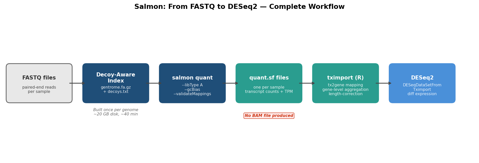

The parameters that matter for standard RNA-seq:

Step 3: QC Checks on Mapping Rates

After quantification, check the mapping rate for every sample before proceeding. A healthy Salmon mapping rate for a standard poly(A)-selected human RNA-seq library against a GENCODE transcriptome is typically between 80 and 95 percent. Rates below 70 percent are a warning sign worth investigating.

# Extract mapping rates from all samples
for SAMPLE in $(ls salmon_output/); do
    RATE=$(grep "Mapping rate" salmon_output/${SAMPLE}/logs/salmon_quant.log \
           | awk '{print $NF}')
    echo "${SAMPLE}: ${RATE}"
done

# Parse mapping rates in R for plotting
mapping_rates <- data.frame(
  sample = c("sample_01", "sample_02", "sample_03",
             "sample_04", "sample_05", "sample_06"),
  rate   = c(91.2, 90.8, 88.4, 92.1, 89.7, 91.5)  # replace with actual values
)

# Flag samples below threshold
threshold <- 80
mapping_rates$flag <- ifelse(mapping_rates$rate < threshold, "LOW", "OK")

cat("Samples with mapping rate below", threshold, "%:\n")
print(mapping_rates[mapping_rates$flag == "LOW", ])

Low mapping rates have three common causes: high rRNA contamination (the reads map to the genome but not to annotated mRNA transcripts), FASTQ files from a different organism than the index, or a transcriptome-genome version mismatch (GENCODE release 45 transcriptome paired with a GRCh38.p13 genome rather than GRCh38.p14). The last cause is particularly insidious because it often gives a plausible-looking mapping rate slightly below expectations rather than a catastrophic failure.

Step 4: Build the tx2gene Mapping Table

tximport aggregates transcript-level Salmon output to gene-level counts. It needs a two-column mapping from transcript IDs to gene IDs. The cleanest way to build this from GENCODE annotation is with the txdbmaker or tximeta package:

# Option 1: Build tx2gene from the GTF with txdbmaker (Bioconductor)
if (!requireNamespace("BiocManager", quietly = TRUE))
    install.packages("BiocManager")
BiocManager::install("txdbmaker")

library(txdbmaker)

txdb <- txdbmaker::makeTxDbFromGFF(
    "gencode.v45.annotation.gtf.gz",
    format = "gtf"
)

k <- keys(txdb, keytype = "TXNAME")
tx2gene <- select(txdb,
                  keys     = k,
                  columns  = c("TXNAME", "GENEID"),
                  keytype  = "TXNAME")

# tx2gene should have two columns: TXNAME (transcript ID) and GENEID (gene ID)
head(tx2gene)

# Option 2: Extract directly from GTF with a simple parse (faster, no TxDb)
library(dplyr)

gtf_lines <- readLines(gzcon(file("gencode.v45.annotation.gtf.gz", "rb")))
tx_lines  <- gtf_lines[grepl('\ttranscript\t', gtf_lines)]

tx2gene <- data.frame(
    TXNAME = sub('.*transcript_id "([^"]+)".*', '\\1', tx_lines),
    GENEID = sub('.*gene_id "([^"]+)".*', '\\1', tx_lines)
) |>
    dplyr::distinct() |>
    dplyr::mutate(
        # Strip version numbers to match --gencode flag in salmon index
        TXNAME = sub("\\.\\d+$", "", TXNAME),
        GENEID = sub("\\.\\d+$", "", GENEID)
    )

dim(tx2gene)   # should be ~250,000 rows for GENCODE 45 human
head(tx2gene)

Step 5: Import with tximport and Feed into DESeq2

tximport by Soneson, Love, and Robinson (2015, F1000Research) handles the transcript-to-gene aggregation and produces a length-correction offset matrix that accounts for differential isoform usage across samples. This offset is important: without it, a gene that switches from a long isoform to a short isoform may appear downregulated in a naive count analysis simply because shorter transcripts generate fewer fragments at equal expression.

library(tximport)
library(DESeq2)

# List the quant.sf files in sample order matching your metadata
quant_files <- file.path(
    "salmon_output",
    c("sample_01", "sample_02", "sample_03",
      "sample_04", "sample_05", "sample_06"),
    "quant.sf"
)
names(quant_files) <- c("sample_01", "sample_02", "sample_03",
                         "sample_04", "sample_05", "sample_06")

# Verify all files exist before importing
stopifnot(all(file.exists(quant_files)))

# Import with tximport
# type = "salmon" reads the quant.sf format
# tx2gene: transcript-to-gene mapping built above
# countsFromAbundance = "lengthScaledTPM": recommended for DESeq2 (offsets for isoform switching)
txi <- tximport(
    quant_files,
    type                = "salmon",
    tx2gene             = tx2gene,
    countsFromAbundance = "lengthScaledTPM",
    ignoreTxVersion     = TRUE   # matches --gencode stripping in index
)

# Inspect the output
dim(txi$counts)       # genes x samples
dim(txi$abundance)    # same: TPM values
summary(colSums(txi$counts))   # library sizes should be in the millions

# Load metadata
metadata <- data.frame(
    condition = factor(c("control", "control", "control",
                          "treated", "treated", "treated"),
                        levels = c("control", "treated")),
    row.names = names(quant_files)
)

# Build DESeqDataSet directly from tximport output
# Note: use DESeqDataSetFromTximport, NOT DESeqDataSetFromMatrix
dds <- DESeqDataSetFromTximport(
    txi      = txi,
    colData  = metadata,
    design   = ~ condition
)

# Pre-filter
dds <- dds[rowSums(counts(dds)) >= 10, ]

# Run DESeq2
dds <- DESeq(dds)
res <- results(dds, name = "condition_treated_vs_control")
summary(res)

The DESeqDataSetFromTximport function (not DESeqDataSetFromMatrix) is the correct constructor when coming from tximport. It automatically incorporates the offset matrix that corrects for effective gene length differences across samples. Using DESeqDataSetFromMatrix on the txi$counts object directly discards this offset, removing one of the key advantages of the Salmon-tximport pipeline.

The post DESeq2 vignette on tximport integration at Bioconductor, maintained by Michael Love’s group, is the authoritative reference for this specific workflow. The tximport vignette by Soneson and Love documents the countsFromAbundance options and their statistical implications. Both are worth bookmarking.

Final Sanity Checks

Before proceeding to differential expression, run three sanity checks:

# 1. Are library sizes consistent across samples?
# Large discrepancies (>5x) warrant investigation
colSums(counts(dds)) |> sort()

# 2. Do samples cluster by condition on PCA?
vsd <- vst(dds, blind = TRUE)
plotPCA(vsd, intgroup = "condition")

# 3. Is the mapping rate consistent with expected library quality?
# (already checked in bash step above, but confirm here)
# If any sample has < 80% mapping rate, investigate before publishing

NotchBio uses this exact Salmon configuration by default: decoy-aware indexing with --gencode flag, quantification with --validateMappings, --gcBias, and --seqBias, tximport with lengthScaledTPM, and DESeqDataSetFromTximport as the DESeq2 entry point. The mapping rate for every sample is reported in the run summary before differential expression begins, and any sample below 75 percent mapping rate triggers a warning that blocks the analysis until you confirm how to proceed.

Related Reading

• STAR vs Salmon vs HISAT2: When To Use Each (With Working Code)
• fastp vs Trimmomatic vs BBDuk: A Benchmark on RNA-Seq Reads
• GTF and GFF Files: Why They Hurt and How To Tame Them
• How to Build a Salmon Index and Quantify Bulk RNA-Seq Reads