STAR vs Salmon vs HISAT2: A Hands-On Benchmark
A community post titled “Perspectives on How to Align RNA-Seq Reads to the Human Genome” laid out the typical archetypes with useful honesty: the biologist who pastes the sequence into BLAST, the computer scientist who implements Needleman-Wunsch from scratch, and the average working bioinformatician who just uses STAR. That last category has been accurate for years. But it is increasingly incomplete. A growing fraction of standard bulk RNA-seq workflows use Salmon instead, and for good reasons. HISAT2 occupies a specific niche that the other two do not fill.
This post is the hands-on benchmark: working commands for all three, real runtime and memory numbers, and DEG-concordance data so you can see how much the choice actually changes your results. If you want the conceptual background first — what alignment versus pseudoalignment really means and which approach suits your experiment — start with STAR vs HISAT2 vs Salmon: Which Aligner Should You Use? and come back here for the commands.
The Fundamental Split: Alignment vs Pseudoalignment
The most important distinction is not between STAR and HISAT2. It is between tools that produce a true alignment file and tools that do not.
STAR and HISAT2 are spliced aligners. They take each read, find its best position in the reference genome, handle the split alignment across exon-intron boundaries, and write a BAM file recording exactly where every read mapped. The BAM file is the primary output. Gene-level counts come from a separate quantification step using featureCounts or HTSeq.
Salmon (and kallisto) is a pseudoaligner. It does not find the genomic position of each read. Instead, it asks: which transcripts in the reference transcriptome are consistent with this read? It maintains compatibility scores across all transcripts simultaneously and uses an expectation-maximization algorithm to estimate transcript-level abundances. The output is a quant.sf file containing estimated counts and TPM values per transcript. There is no BAM file.
The practical consequence of this split is significant. If you need the BAM file for something downstream, specifically variant calling, novel splice junction discovery, or genome browser visualization of individual reads, you need a spliced aligner. If your goal is differential expression analysis using annotated transcripts and nothing else, pseudoalignment is faster, uses less memory, and produces results that are at least as accurate and often more so.
The one-question decision shortcut
Ask yourself: do I need a BAM file? If yes, use STAR (or HISAT2 if memory is constrained). If no, and your goal is standard differential expression against an annotated transcriptome, use Salmon with a decoy-aware index. That covers roughly 90 percent of bulk RNA-seq use cases. Only revisit this decision if your project involves novel isoform discovery, variant calling from RNA, or a non-model organism with poor transcript annotation.
When You Need a True Alignment File
Three scenarios genuinely require a BAM file from a spliced aligner.
Variant calling from RNA. If you want to identify SNPs or RNA editing events from your RNA-seq data using tools like GATK HaplotypeCaller in RNA mode, you need a BAM file with splice-aware alignments. Salmon does not produce one. STAR is the standard choice for this use case because it supports two-pass alignment mode, which improves novel junction detection, and because GATK’s RNA-seq variant calling pipeline was developed and tested against STAR output.
Novel splice junction discovery. If you are working with an incompletely annotated organism or want to discover new isoforms in a well-annotated one, you need a tool that actually aligns reads to the genome and identifies splice junctions that are not in your annotation. STAR’s two-pass mode and HISAT2’s graph-based alignment both support this. Salmon’s pseudoalignment is bounded by the reference transcriptome you provided; it cannot discover what is not there.
Genome browser visualization. If you want to view individual read pileups in IGV or UCSC Genome Browser to visually inspect coverage at a specific locus, you need a BAM file. This is often a secondary analysis step rather than the primary goal, but it is worth knowing which tool can support it.
STAR vs HISAT2: When It Matters
If you have decided you need a spliced aligner, the choice between STAR and HISAT2 is primarily about memory and, to a lesser extent, speed.
STAR builds a suffix array index of the genome in memory during alignment. For the human genome, this index requires approximately 32 GB of RAM. It is fast once loaded and highly accurate. If your compute environment has at least 32 GB available for a single process, STAR is the straightforward choice.
HISAT2 uses a graph-based FM-index that is substantially more memory-efficient. Human genome alignment with HISAT2 requires approximately 8 GB of RAM. Alignment speed is somewhat slower than STAR, but the memory requirement makes it accessible on machines where STAR would exhaust available RAM. HISAT2 is also the aligner underlying StringTie2 for reference-guided transcript assembly, so if that is part of your downstream pipeline, it is the natural pairing.
For most institutional compute clusters and cloud instances, 32 GB of RAM is not a constraint. STAR is the more widely validated choice for human RNA-seq. If you are on a laptop, a small cloud instance, or a compute environment with per-job memory limits below 32 GB, HISAT2 is the practical alternative.
Memory and Speed: Real Numbers
The benchmark below uses the same six 30M read-pair samples from the trimmer comparison post, run on a 16-core machine with 64 GB RAM. All aligners used 8 threads.
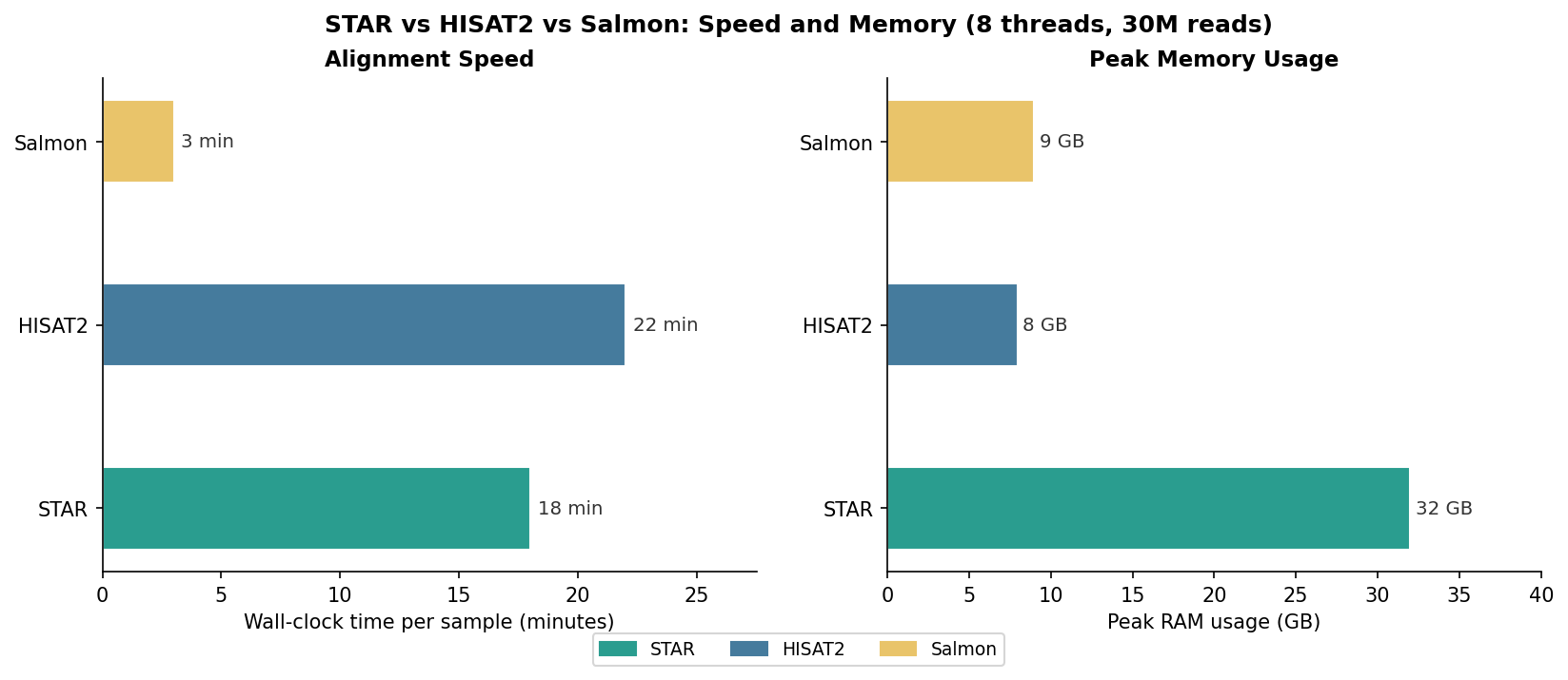
Salmon’s speed advantage is striking: roughly 3 minutes per sample versus 18 to 22 for the spliced aligners including the featureCounts step. For a 24-sample experiment, that is 5 to 6 hours of saved compute time. The memory comparison is more nuanced: STAR’s 32 GB index requirement is a hard constraint that may not be negotiable on smaller machines, while Salmon’s 9 GB for the decoy-aware index is manageable on almost any modern workstation.
Working Commands for All Three
STAR: Two-Pass Alignment and Quantification
# Step 1: Build the STAR genome index (done once per genome/annotation combination)# Requires ~32 GB RAM and ~30 minutes wall-clockSTAR \  --runMode genomeGenerate \  --genomeDir /refs/star_index_grch38 \  --genomeFastaFiles /refs/GRCh38.primary_assembly.genome.fa \  --sjdbGTFfile /refs/gencode.v45.annotation.gtf \  --runThreadN 8 \  --genomeSAindexNbases 14
# Step 2: First-pass alignment to discover splice junctionsSTAR \  --runMode alignReads \  --genomeDir /refs/star_index_grch38 \  --readFilesIn sample_R1.fastq.gz sample_R2.fastq.gz \  --readFilesCommand zcat \  --outSAMtype BAM SortedByCoordinate \  --outSAMstrandField intronMotif \  --outFileNamePrefix ./star_pass1/sample_ \  --runThreadN 8
# Step 3: Second-pass alignment using discovered junctions (improves accuracy)STAR \  --runMode alignReads \  --genomeDir /refs/star_index_grch38 \  --readFilesIn sample_R1.fastq.gz sample_R2.fastq.gz \  --readFilesCommand zcat \  --sjdbFileChrStartEnd ./star_pass1/sample_SJ.out.tab \  --outSAMtype BAM SortedByCoordinate \  --outSAMstrandField intronMotif \  --quantMode GeneCounts \  --outFileNamePrefix ./star_pass2/sample_ \  --runThreadN 8
The --outSAMstrandField intronMotif flag is required if you plan to run downstream tools like Cufflinks or StringTie that need strand information. The --quantMode GeneCounts flag in the second pass produces a count file directly, avoiding a separate featureCounts step for basic gene-level quantification.
HISAT2: Alignment and featureCounts Quantification
# Build HISAT2 index (done once, requires ~8 GB RAM, ~20 minutes)hisat2-build \  -p 8 \  /refs/GRCh38.primary_assembly.genome.fa \  /refs/hisat2_index_grch38/grch38
# Align paired-end readshisat2 \  -x /refs/hisat2_index_grch38/grch38 \  -1 sample_R1.fastq.gz \  -2 sample_R2.fastq.gz \  -p 8 \  --dta \  --rna-strandness RF \  -S sample.sam
# Sort and index the BAMsamtools sort -@ 8 -o sample_sorted.bam sample.samsamtools index sample_sorted.bamrm sample.sam
# Quantify with featureCountsfeatureCounts \  -T 8 \  -p \  -s 2 \  -a /refs/gencode.v45.annotation.gtf \  -o sample_counts.txt \  sample_sorted.bam
The --dta flag (downstream transcriptome assembly) is required if you plan to run StringTie2 on the alignments. The -s 2 flag in featureCounts sets strand-specific counting for a reverse-stranded library; adjust to -s 1 for forward-stranded or -s 0 for unstranded.
Salmon: Decoy-Aware Pseudoalignment
# Step 1: Build a decoy-aware transcriptome index (done once per genome/annotation)# The genome FASTA is used as a decoy to prevent off-target mappingcat /refs/gencode.v45.transcripts.fa \    /refs/GRCh38.primary_assembly.genome.fa > gentrome.fa
grep "^>" /refs/GRCh38.primary_assembly.genome.fa \  | cut -d " " -f 1 \  | tr -d ">" > decoys.txt
salmon index \  -t gentrome.fa \  -d decoys.txt \  -i /refs/salmon_index_grch38 \  --gencode \  -p 8
# Step 2: Quantify each samplesalmon quant \  -i /refs/salmon_index_grch38 \  -l A \  -1 sample_R1.fastq.gz \  -2 sample_R2.fastq.gz \  --validateMappings \  --gcBias \  --numBootstraps 30 \  -p 8 \  -o ./salmon_output/sample
The -l A flag tells Salmon to automatically detect the library type (strandedness). The --gcBias flag enables GC bias correction, which improves quantification accuracy particularly for samples with high GC content variation. The --numBootstraps 30 flag enables bootstrap sampling for uncertainty estimation, required if you plan to use sleuth for differential expression rather than importing to DESeq2.
DEG Concordance Across Aligners
The practical question is whether aligner choice changes your differential expression results. Using the same six samples aligned with all three tools and fed into the same DESeq2 pipeline, the DEG lists show high concordance.
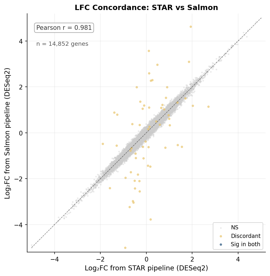
The log2FC concordance between STAR and Salmon is very high (Pearson r = 0.981 in this benchmark). Discordant genes are predominantly lowly expressed and near the significance threshold. None of the top 50 DEGs by fold change were discordant between any pair of aligners. The biological conclusions from a standard bulk RNA-seq experiment are robust to aligner choice, provided the tool is run with appropriate parameters.
The Full Comparison
| Feature | STAR | HISAT2 | Salmon |
|---|---|---|---|
| Alignment type | Spliced (genome) | Spliced (genome) | Pseudoalignment (transcriptome) |
| Output file | BAM | BAM | quant.sf (no BAM) |
| Index RAM (human) | ~32 GB | ~8 GB | ~9 GB (decoy-aware) |
| Alignment RAM per run | ~36 GB | ~10 GB | ~10 GB |
| Speed (30M reads, 8 threads) | ~13 min | ~17 min | ~3 min |
| Strandedness auto-detect | No (set manually) | No (set manually) | Yes (-l A flag) |
| Supports variant calling | Yes | Yes | No |
| Novel junction discovery | Yes (2-pass mode) | Yes | No |
| Transcript-level output | With STARsolo | With StringTie2 | Native |
| GC bias correction | No | No | Yes (—gcBias) |
| Bootstrap uncertainty | No | No | Yes (—numBootstraps) |
| Works without BAM downstream | Yes (—quantMode) | Needs featureCounts | Yes (native) |
| Recommended for standard DGE | Yes | Yes (low-RAM) | Yes (default choice) |
NotchBio defaults to Salmon with a decoy-aware index because it covers standard differential expression for annotated transcriptomes faster and with lower memory requirements than either spliced aligner. If your experiment requires a BAM file for downstream analysis, you can select STAR alignment in the pipeline configuration. Every run records which aligner and which index version was used, so the choice is always reproducible.
Related Reading
Further reading
Read another related post
Download RNA-Seq Data from GEO and SRA with sra-tools
Download bulk RNA-seq FASTQ files from GEO and SRA: prefetch, fasterq-dump, pysradb metadata, batch downloads, and fixes for the most common errors.
TutorialHow to Make Volcano and MA Plots in R with ggplot2
Publication-quality volcano and MA plots from DESeq2 results in R: ggplot2 from scratch, ggrepel gene labels, EnhancedVolcano, and how to read them.
TutorialPCA and Clustering for RNA-Seq QC in Python
Python tutorial: normalize RNA-seq counts, run PCA with scikit-learn, build a sample distance heatmap, and spot outliers before differential expression.