How to Run STAR Alignment for Bulk RNA-Seq (Step-by-Step)
Salmon is faster and needs less RAM, but STAR gives you something Salmon cannot: actual genome coordinates for every read.
If your project involves visualizing alignments in IGV, calling splice junctions, detecting novel transcripts, or feeding a BAM file into a ChIP-seq or ATAC-seq pipeline alongside your RNA-seq, STAR is the right tool. The BAM output is the real deliverable. Gene counts are a side product.
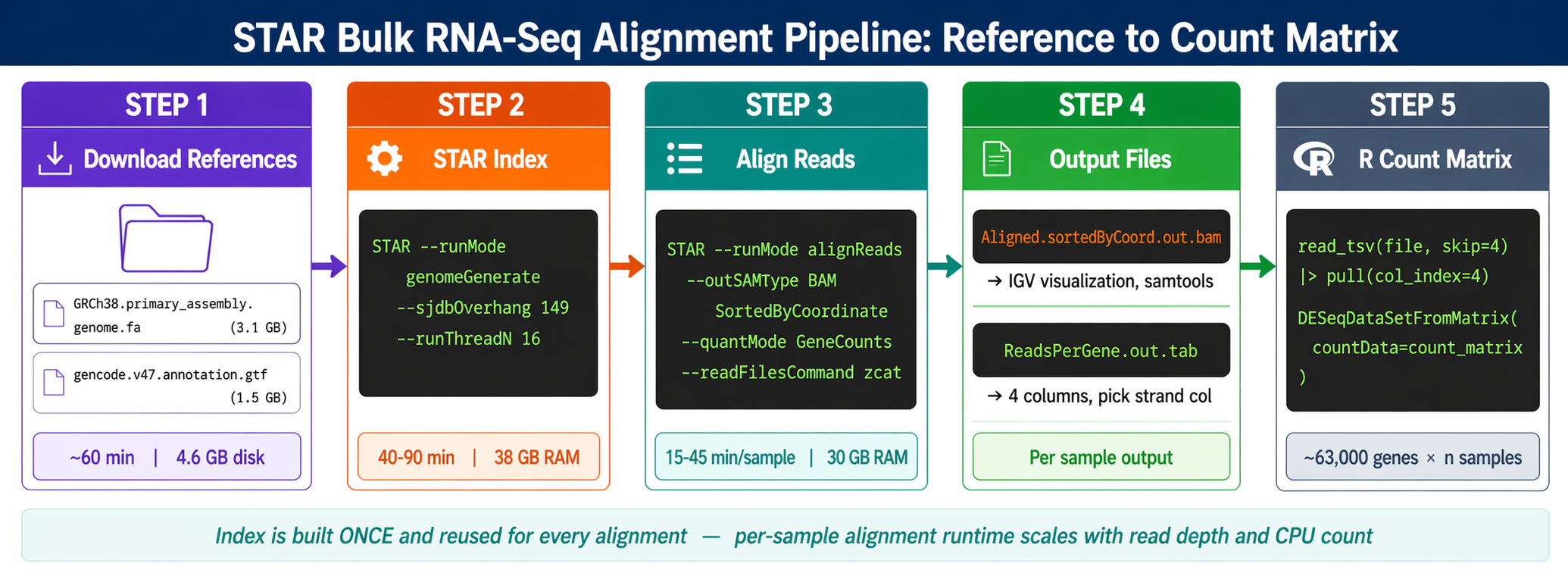
This tutorial covers the full STAR workflow for bulk RNA-seq: downloading the GENCODE reference, building a genome index with the correct --sjdbOverhang value, aligning paired-end trimmed reads, extracting gene counts from ReadsPerGene.out.tab, and assembling the count matrix in R for DESeq2. We use the trimmed reads from the FASTQ quality control tutorial and the r-rnaseq conda environment from the Ubuntu and macOS setup guide.
When to Use STAR Instead of Salmon
Salmon wins on speed and simplicity for standard differential expression. STAR wins when you need genome-level output.
Use STAR when:
- You want to visualize alignments in IGV or UCSC to confirm expression patterns
- Your lab processes RNA-seq alongside ATAC-seq or ChIP-seq and needs consistent BAM pipelines
- You are doing splice junction analysis or looking for novel isoforms
- A collaborator or reviewer specifically asks for genome-aligned data
- You are using RSEM downstream for isoform-level quantification
Use Salmon (covered in How to Build a Salmon Index and Quantify Bulk RNA-Seq Reads) when you only need gene-level counts for differential expression and want results in under an hour per sample.
The counts you get from STAR --quantMode GeneCounts and Salmon quant agree closely at the gene level for most experiments. The choice is primarily about what else you need from the data.
RAM requirement: STAR needs 38 GB for the human genome index
Building a STAR genome index for the full human genome (GRCh38) requires approximately 38 GB of RAM at peak. Running alignments requires around 30 GB. This is non-negotiable. If your workstation has 16 GB, you cannot run STAR on the full human genome locally. Use a university HPC cluster, a cloud VM, or switch to Salmon for your analysis.
How to Download the GENCODE Reference Files
STAR needs two files: the primary genome assembly FASTA and the annotation GTF.
We use GENCODE v47 to match the Salmon reference from the Salmon indexing tutorial. Using the same annotation version across your entire pipeline is important for consistent gene ID handling.
mkdir -p references/star && cd references
# Genome primary assembly FASTAwget "https://ftp.ebi.ac.uk/pub/databases/gencode/Gencode_human/release_47/GRCh38.primary_assembly.genome.fa.gz"
# Gene annotation GTFwget "https://ftp.ebi.ac.uk/pub/databases/gencode/Gencode_human/release_47/gencode.v47.annotation.gtf.gz"
# Decompress both (STAR does not accept .gz directly for index building)gunzip GRCh38.primary_assembly.genome.fa.gzgunzip gencode.v47.annotation.gtf.gz
echo "References downloaded and decompressed."ls -lh GRCh38.primary_assembly.genome.fa gencode.v47.annotation.gtf# GRCh38.primary_assembly.genome.fa  ~3.1 GB# gencode.v47.annotation.gtf         ~1.5 GB
For mouse (GRCm39), replace the URLs with the GENCODE mouse equivalents using release M34.
How to Build a STAR Genome Index
The index is built once per reference version. Budget 40 to 90 minutes and 38 GB of RAM.
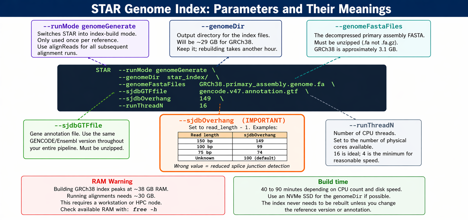
The critical parameter is --sjdbOverhang. It tells STAR the maximum possible overhang on one side of a splice junction.
The --sjdbOverhang option usually equals the minimum read length minus one. It tells STAR what is the maximum possible stretch of sequence that can be found on one side of a splicing site. For most modern datasets with 150 bp paired-end reads, use 149. For 100 bp reads, use 99.
In most cases, the default value of 100 will work similarly to the ideal value if your reads are longer than 100 bp. If your reads are exactly 150 bp, setting it to 149 is marginally more accurate than leaving it at 100.
# Set paths as variables to keep the command readableGENOME_FA="references/GRCh38.primary_assembly.genome.fa"GTF="references/gencode.v47.annotation.gtf"INDEX_DIR="references/star_index_gencode_v47"THREADS=16
mkdir -p "$INDEX_DIR"
STAR \    --runMode          genomeGenerate \    --genomeDir        "$INDEX_DIR" \    --genomeFastaFiles "$GENOME_FA" \    --sjdbGTFfile      "$GTF" \    --sjdbOverhang     149 \    --runThreadN       "$THREADS"
echo "Genome index built in $INDEX_DIR"ls -lh "$INDEX_DIR"
STAR prints progress as it runs. The index directory will contain around 29 GB of binary files. Do not delete it after the first use.
Save the exact STAR version and sjdbOverhang in your methods
Your methods section must report the STAR version, reference genome, annotation version, and the --sjdbOverhang value used. Run STAR --version and record the output. Reviewers increasingly check whether index parameters match the stated read length.
How to Run STAR Alignment on Paired-End RNA-Seq Reads
With the index ready, each sample alignment takes 15 to 45 minutes depending on sequencing depth and CPU count.
Single sample alignment
INDEX_DIR="references/star_index_gencode_v47"TRIM_DIR="results/trimmed"STAR_DIR="results/star"THREADS=16
mkdir -p "$STAR_DIR" logs
# Align one sampleSAMPLE="SRR26891234"R1="${TRIM_DIR}/${SAMPLE}_1.trimmed.fastq.gz"R2="${TRIM_DIR}/${SAMPLE}_2.trimmed.fastq.gz"PREFIX="${STAR_DIR}/${SAMPLE}_"
STAR \    --runMode              alignReads \    --genomeDir            "$INDEX_DIR" \    --readFilesIn          "$R1" "$R2" \    --readFilesCommand     zcat \    --outFileNamePrefix    "$PREFIX" \    --outSAMtype           BAM SortedByCoordinate \    --quantMode            GeneCounts \    --runThreadN           "$THREADS" \    --outSAMunmapped       Within \    --outSAMattributes     Standard \    2>&1 | tee "logs/star_${SAMPLE}.log"
What each flag does
--readFilesCommand zcat is required for gzipped inputs. Without it, STAR tries to read the compressed bytes directly and produces garbage.
--outSAMtype BAM SortedByCoordinate writes a coordinate-sorted BAM file, which is required for visualization in IGV and for samtools indexing. Do not use Unsorted; sorting later with samtools costs extra time and disk.
--quantMode GeneCounts tells STAR to count reads per gene simultaneously with alignment. A read is counted if it overlaps one and only one gene by at least one base. Both ends of the paired-end read are checked for overlaps. The counts coincide with those produced by htseq-count with default parameters.
--outSAMunmapped Within retains unmapped reads inside the BAM file, which is useful for diagnosing low mapping rates without needing the raw FASTQ.
Align all samples in a loop
#!/bin/bashset -euo pipefail
INDEX_DIR="references/star_index_gencode_v47"TRIM_DIR="results/trimmed"STAR_DIR="results/star"THREADS=16
mkdir -p "$STAR_DIR" logs
for R1 in "$TRIM_DIR"/*_1.trimmed.fastq.gz; do    SAMPLE=$(basename "$R1" _1.trimmed.fastq.gz)    R2="${TRIM_DIR}/${SAMPLE}_2.trimmed.fastq.gz"    PREFIX="${STAR_DIR}/${SAMPLE}_"
    echo "[$(date +%H:%M:%S)] Aligning $SAMPLE"
    STAR \        --runMode           alignReads \        --genomeDir         "$INDEX_DIR" \        --readFilesIn       "$R1" "$R2" \        --readFilesCommand  zcat \        --outFileNamePrefix "$PREFIX" \        --outSAMtype        BAM SortedByCoordinate \        --quantMode         GeneCounts \        --runThreadN        "$THREADS" \        --outSAMunmapped    Within \        --outSAMattributes  Standard \        2>&1 | tee "logs/star_${SAMPLE}.log"
    # Index the BAM for IGV visualization    samtools index "${PREFIX}Aligned.sortedByCoord.out.bam"
    echo "[$(date +%H:%M:%S)] Done: $SAMPLE"done
echo "All samples aligned."
Run it:
bash star_align_all.shFor a 12-sample experiment at 50 million reads per sample, this runs for roughly 6 to 8 hours on a 16-core machine. This is the main reason teams move STAR pipelines to HPC clusters or cloud compute.
How to Read STAR Output Files
Each sample produces a directory of files. The two you care about most are the BAM and the gene counts table.
results/star/SRR26891234_Aligned.sortedByCoord.out.bam # genome alignmentresults/star/SRR26891234_Log.final.out # alignment statisticsresults/star/SRR26891234_ReadsPerGene.out.tab # gene countsresults/star/SRR26891234_SJ.out.tab # splice junctionsReading the alignment log
The Log.final.out file is the most important QC output.
cat "results/star/SRR26891234_Log.final.out"Key lines to check:
Number of input reads | 45,123,456Uniquely mapped reads % | 91.42%Reads mapped to multiple loci % | 4.23%Reads unmapped: too short % | 2.18%Reads unmapped: other % | 2.17%Unique mapping rates above 80% are acceptable. Above 85% is good. Rates consistently below 70% across samples indicate a mismatch between the reads and the reference, likely a wrong species, heavy rRNA contamination, or adapter sequences that were not trimmed.
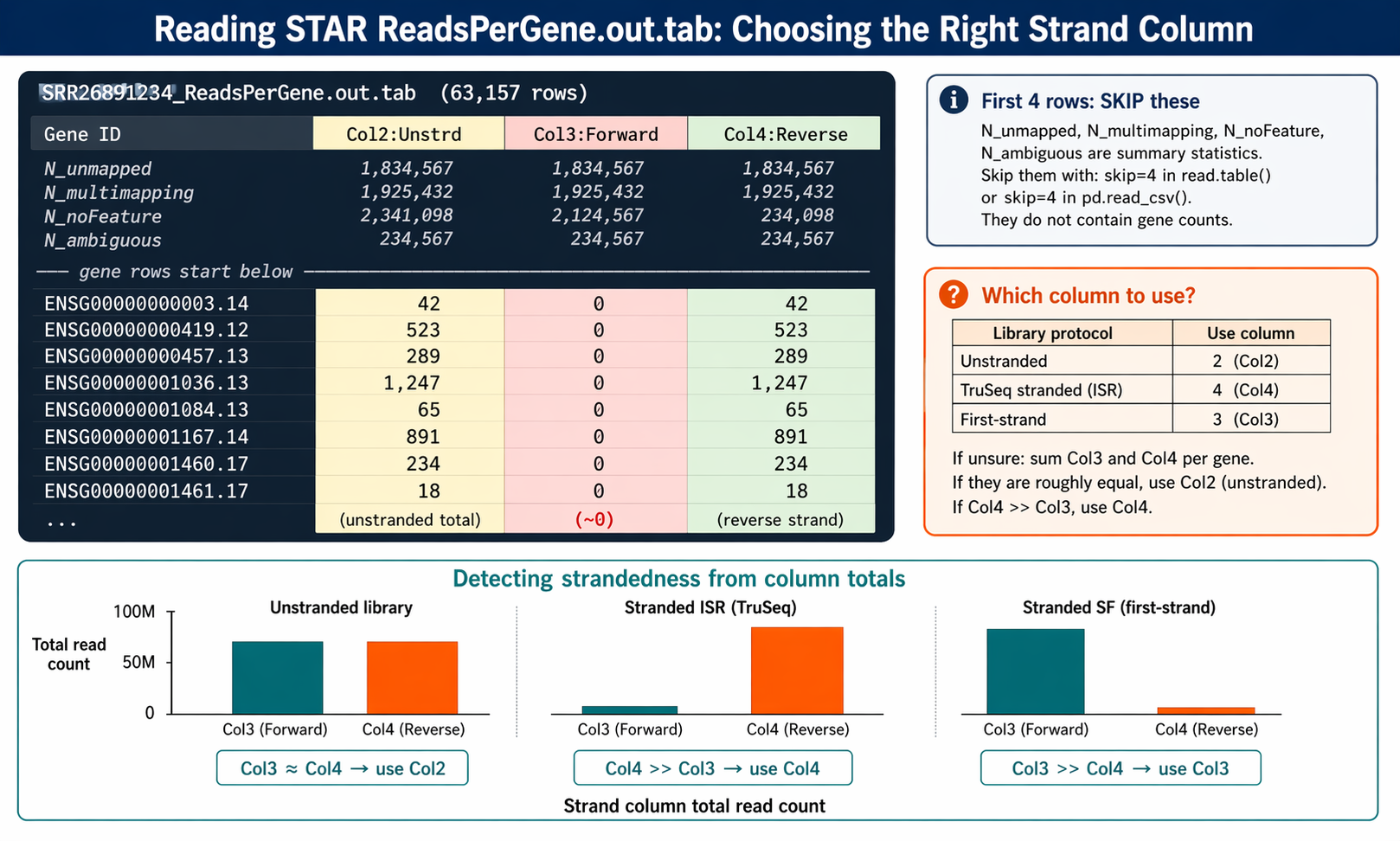
Reading the ReadsPerGene.out.tab file
head -5 "results/star/SRR26891234_ReadsPerGene.out.tab"N_unmapped 1834567 1834567 1834567N_multimapping 1925432 1925432 1925432N_noFeature 2341098 2124567 234098N_ambiguous 234567 234567 234567ENSG00000000003.14 42 0 42The first four rows are summary statistics for unmapped, multimapping, no-feature, and ambiguous reads. From row 5 onward, each row is a gene with four columns: gene ID, unstranded count, forward-strand count, and reverse-strand count.
Column 2 gives counts for unstranded RNA-seq. Column 3 gives counts for the first read strand aligned with RNA. Column 4 gives counts for the second read strand aligned with RNA (the reverse complement strand).
For standard Illumina TruSeq stranded libraries (ISR protocol), use column 4. For unstranded libraries, use column 2. If you are unsure, check the counts in columns 3 and 4. If they are roughly equal, your library is unstranded. If one is dramatically larger, your library is stranded and you should use the larger column.
How to Load STAR Counts into R and Build a DESeq2 Matrix
This step assembles all per-sample ReadsPerGene.out.tab files into a single gene-by-sample count matrix, then hands it off to DESeqDataSetFromMatrix.
library(dplyr)library(readr)library(DESeq2)
# ── 1. List all ReadsPerGene files ───────────────────────────────────star_dir    <- "results/star"count_files <- list.files(star_dir,                          pattern    = "ReadsPerGene.out.tab",                          full.names = TRUE)
# Derive sample names from file pathssample_names <- sub("_ReadsPerGene.out.tab", "",                    basename(count_files))
# ── 2. Load and combine ──────────────────────────────────────────────# STAR tab files have 4 columns; skip the first 4 summary rows# Column index for counts:#   2 = unstranded, 3 = forward strand, 4 = reverse strand (TruSeq stranded)STRAND_COLUMN <- 4   # adjust to 2 for unstranded libraries
load_star_counts <- function(file_path, col_index) {  read_tsv(file_path,           col_names = c("gene_id", "unstranded", "forward", "reverse"),           skip       = 4,         # skip N_unmapped, N_multi, N_noFeature, N_ambiguous           col_types  = "ciii") |>    pull(col_index)               # extract just the count vector}
# Build the count matrix: rows = genes, columns = samplesgene_ids     <- read_tsv(count_files[1],                         col_names = c("gene_id","u","f","r"),                         skip = 4, col_types = "ciii")$gene_id
count_matrix <- sapply(count_files, load_star_counts,                       col_index = STRAND_COLUMN)rownames(count_matrix) <- gene_idscolnames(count_matrix) <- sample_names
cat("Count matrix dimensions:", dim(count_matrix), "\n")# Genes: ~63,000 for GENCODE v47 (including non-coding)
# ── 3. Verify column totals are plausible ────────────────────────────cat("Reads per sample (selected column):\n")print(colSums(count_matrix))
Build the DESeqDataSet
# Load sample metadatametadata <- read_csv("sample_sheet.csv") |>  column_to_rownames("sample_id") |>  filter(rownames(.) %in% sample_names)
# Align order of samples between matrix and metadatacount_matrix <- count_matrix[, rownames(metadata)]
# Build DESeqDataSetdds <- DESeqDataSetFromMatrix(  countData = count_matrix,  colData   = metadata,  design    = ~ condition)
# Set reference level and filter low countsdds$condition      <- relevel(dds$condition, ref = "control")keep <- rowSums(counts(dds) >= 10) >= 3dds  <- dds[keep, ]
cat("Genes after filtering:", nrow(dds), "\n")# Proceed with DESeq() as in the DESeq2 tutorial
From here, the DESeq2 analysis is identical to the tximeta-based approach in the DESeq2 tutorial. The count matrix is the same data structure either way.
How to Collect Alignment Statistics Across All Samples
Before running DESeq2, review the alignment summary across all samples. A single outlier sample with low unique mapping can distort your results.
# Extract key alignment stats from every Log.final.outecho -e "sample\ttotal_reads\tunique_map_pct\tmultimap_pct\tunmapped_short_pct" \    > results/star/alignment_summary.tsv
for log in results/star/*Log.final.out; do    sample=$(basename "$log" _Log.final.out)    total=$(grep "Number of input reads"       "$log" | awk '{print $NF}')    unique=$(grep "Uniquely mapped reads %"    "$log" | awk '{print $NF}')    multi=$(grep "% of reads mapped to multiple" "$log" | awk '{print $NF}')    short=$(grep "unmapped: too short"         "$log" | awk '{print $NF}')    echo -e "${sample}\t${total}\t${unique}\t${multi}\t${short}"done >> results/star/alignment_summary.tsv
cat results/star/alignment_summary.tsv
Add this summary to your MultiQC report by running MultiQC over the results directory:
multiqc results/star/ results/fastqc_trimmed/ \ --outdir results/multiqc/ \ --filename "full_pipeline_QC.html"MultiQC automatically detects STAR log files and adds an alignment statistics section.
Manual STAR Pipeline vs NotchBio
STAR is a solid, reproducible aligner. It is also the slowest and most memory-intensive step in any RNA-seq pipeline.
Building the index demands 38 GB of RAM and roughly an hour of compute. Each sample alignment takes 15 to 45 minutes. A 12-sample experiment can run for an entire working day before you touch the count matrix.
NotchBio runs STAR and Salmon in parallel on cloud infrastructure, eliminating the index RAM barrier entirely.
| Step | Manual STAR Pipeline | NotchBio |
|---|---|---|
| Download genome + GTF | ~60 min for GRCh38, ~4.6 GB disk | Not required |
| Build STAR index | 40-90 min, 38 GB RAM peak | Pre-built, all GENCODE/Ensembl versions |
| Align all samples | 15-45 min per sample, sequential | Parallel cloud execution |
| Check Log.final.out | Manual grep loop or MultiQC | Auto-added to QC dashboard |
| Assemble count matrix | R loop over ReadsPerGene files | Automatic |
| Choose strandedness column | Manual: check col 3 vs col 4 | Auto-detected per sample |
| Index BAM files | samtools index after each alignment | Included, downloadable |
| MultiQC integration | Re-run multiqc results/star/ | Auto-populated in report |
| RAM requirement | 38 GB for index, 30 GB for alignment | None, runs on our infrastructure |
| Total wall time | 6-10 hours for 12 samples | 30-60 min in parallel |
If your project requires genome-level BAM files, STAR is the right choice. If you only need counts for differential expression and do not need IGV-ready alignments, notchbio.app runs Salmon quantification with pre-built decoy-aware indices that are faster and require no local RAM. Upload your trimmed FASTQs and select your organism.
Further reading
Read another related post
PCA and Clustering for RNA-Seq QC in Python
Python tutorial: normalize RNA-seq counts, run PCA with scikit-learn, build a sample distance heatmap, and spot outliers before differential expression.
TutorialPyDESeq2 Tutorial: Differential Expression in Python
The complete PyDESeq2 reference in Python: DeseqDataSet, DeseqStats, apeglm shrinkage, multi-factor designs, multiple contrasts, and pandas result filtering.
TutorialHow to Run DESeq2: From Count Matrix to Results
Step-by-step DESeq2 in R: build a DESeqDataSet, understand size factors and dispersion, run DESeq(), interpret the results columns, then shrink and filter DEGs.