Tutorial

Differential Expression Analysis in Python with PyDESeq2: A Complete Tutorial

By Abdullah Shahid · April 15, 2026 · 16 min read

rna-seq tutorial differential-expression

R has owned bulk RNA-seq differential expression for a decade. DESeq2 is the dominant tool, it lives in R, and most tutorials assume you are comfortable with R data structures. If your analysis stack is Python, the standard advice has been to either write a subprocess call to R or re-implement the normalization yourself and accept inferior statistics.

PyDESeq2 changes this. Published in Bioinformatics in 2023, it is a from-scratch Python reimplementation of the DESeq2 workflow, written in pure Python using NumPy and SciPy, with no R dependency anywhere in the call stack (Muzellec et al., 2023). It is part of the scverse ecosystem alongside Scanpy and AnnData, which means it integrates naturally with the Python single-cell and multi-omics tooling that has become standard in modern labs.

This tutorial walks through the complete PyDESeq2 workflow from scratch: installation, input preparation, model fitting, statistical testing, LFC shrinkage, and saving results. It also covers the critical ways PyDESeq2 differs from DESeq2 in R, which are the differences that will catch you if you switch without reading the docs.

For the R-native mental model behind the same statistics, pair this with How DESeq2 Actually Works (Without the Math Overload) and How to Run DESeq2: A Complete Walkthrough from Count Matrix to Results. If your starting point is still the input table, What Is a Count Matrix and Why Does It Matter is the prerequisite refresher.

PyDESeq2 pipeline diagram showing the five steps: load count matrix and metadata as pandas DataFrames, filter low-count genes, create DeseqDataSet and call deseq2(), create DeseqStats with contrast and call summary(), then optionally call lfc_shrink() before accessing results_df — Figure 1: The PyDESeq2 pipeline is split into two classes: DeseqDataSet handles normalization and model fitting, DeseqStats handles hypothesis testing and optional LFC shrinkage. Results live in a standard pandas DataFrame.

What Is PyDESeq2 and How Does It Compare to DESeq2 in R?

PyDESeq2 implements the same negative binomial GLM model as DESeq2. The workflow is identical: estimate size factors, estimate and shrink gene-wise dispersions, fit the GLM, and perform Wald tests. The published benchmarks on eight TCGA datasets show that PyDESeq2 returns very similar sets of significant genes and pathways to DESeq2, while achieving higher model likelihood for dispersion and LFC parameters on the vast majority of genes, at comparable speeds for large cohorts (PMC10502239).

The practical differences that matter for day-to-day use:

Count matrix orientation is transposed. In R DESeq2, the count matrix is genes × samples (rows are genes). In PyDESeq2, the count matrix must be samples × genes (rows are samples, columns are genes). This is the most common source of silent failure when porting from R.

Two-class structure instead of one. DESeq2 in R wraps everything in a single DESeqDataSet. PyDESeq2 separates modeling from testing: DeseqDataSet fits dispersions and LFCs, DeseqStats runs the Wald test and shrinkage.

Results are a pandas DataFrame. Instead of an S4 object you query with accessor functions, ds.results_df is a standard pandas DataFrame you can filter, sort, merge, and plot with the full Python data science toolchain.

Currently implements Wald tests only. Likelihood Ratio Tests (LRT), which are useful for time-course and multi-level experiments, are not yet implemented as of version 0.5. Check the GitHub releases page for current feature status.

Feature	DESeq2 (R)	PyDESeq2 (Python)
Language	R	Python (NumPy, SciPy)
Count matrix orientation	Genes × samples	Samples × genes
Main objects	`DESeqDataSet`	`DeseqDataSet` + `DeseqStats`
Results format	S4 `DESeqResults` object	`pandas.DataFrame` (ds.results_df)
Wald tests	Yes	Yes
Likelihood Ratio Tests	Yes	Not yet
apeglm LFC shrinkage	Yes	Yes
Integration with Python ecosystem	Via rpy2 only	Native
Scverse/AnnData compatible	No	Yes

How to Install PyDESeq2

# Recommended: in a clean conda environment
conda create -n pydeseq2 python=3.11 -y
conda activate pydeseq2

# Install from PyPI
pip install pydeseq2

# Install additional tools used in this tutorial
pip install pandas numpy matplotlib seaborn scikit-learn scipy

Verify the installation:

import pydeseq2
print(pydeseq2.__version__)
# 0.5.4  (or later)

PyDESeq2 is also available through Bioconda (conda install -c bioconda pydeseq2) and is included in the scverse conda channel. Check the PyDESeq2 GitHub for the latest installation instructions, as the package has moved between organizations since its initial release.

How to Prepare Your Count Matrix for PyDESeq2

This is the step most tutorials gloss over, and it is where most errors originate. PyDESeq2 requires:

A count matrix with samples as rows and genes as columns. This is the opposite of the R convention.

Values must be non-negative integers (raw counts, not TPM or normalized values).

The index of the count DataFrame must match the index of the metadata DataFrame exactly.

import pandas as pd
import numpy as np

# ── Option A: Load from featureCounts CSV ──────────────────────
# featureCounts typically outputs genes as rows, samples as columns
counts_raw = pd.read_csv(
    "results/counts/feature_counts.csv",
    index_col = 0  # gene IDs are in column 0
)

# featureCounts format: genes x samples → transpose for PyDESeq2
counts_df = counts_raw.T

print(f"Count matrix shape: {counts_df.shape}")
# (6, 18234)  ← rows=samples, columns=genes

# Verify integer counts
assert (counts_df >= 0).all().all(), "Counts contain negative values"
counts_df = counts_df.astype(int)

# ── Option B: Load from Salmon quant.sf files (Python alternative to tximport) ──
# For each sample, load NumReads column and build the matrix
import os
from pathlib import Path

sample_dirs = sorted(Path("results/salmon").glob("*_quant"))
sample_names = [d.name.replace("_quant", "") for d in sample_dirs]

counts_dict = {}
for name, sdir in zip(sample_names, sample_dirs):
    quant = pd.read_csv(
        sdir / "quant.sf",
        sep   = "\t",
        index_col = "Name",
        usecols   = ["Name", "NumReads"]
    )
    # Round fractional estimated counts to integers
    counts_dict[name] = quant["NumReads"].round().astype(int)

counts_df = pd.DataFrame(counts_dict).T  # samples x genes
print(f"Loaded {counts_df.shape[0]} samples, {counts_df.shape[1]} transcripts")

# ── Build metadata DataFrame ────────────────────────────────────
metadata = pd.DataFrame({
    "condition": ["control", "control", "control",
                  "treated", "treated", "treated"],
    "batch":     ["A",       "A",       "B",
                  "A",       "A",       "B"]
}, index = sample_names)

# Condition must be a string or categorical, not numeric
metadata["condition"] = metadata["condition"].astype(str)
metadata["batch"]     = metadata["batch"].astype(str)

# Verify alignment: sample order must match in both DataFrames
assert list(counts_df.index) == list(metadata.index), \
    "Sample order mismatch between counts and metadata"

print(metadata)
#           condition batch
# ctrl_1      control     A
# ctrl_2      control     A
# ctrl_3      control     B
# treat_1     treated     A
# treat_2     treated     A
# treat_3     treated     B

How to Filter Low-Count Genes Before Running PyDESeq2

Low-count genes add noise without contributing statistical power. Filter them out before model fitting:

# Keep genes with at least 10 total counts across all samples
genes_to_keep = counts_df.columns[counts_df.sum(axis=0) >= 10]
counts_df = counts_df[genes_to_keep]

print(f"Genes after filtering: {counts_df.shape[1]}")
# Before: ~60,000 genes  After: ~18,000-22,000 genes (human, GENCODE)

This threshold is a starting point. For experiments with more replicates, you can be more stringent (e.g., requiring at least 10 counts in at least half the samples). For small experiments, be conservative.

The count matrix orientation in PyDESeq2 is samples × genes, not genes × samples

If you pass a genes × samples matrix to DeseqDataSet, the model will treat each gene as a sample and each sample as a gene. You will not get an error, but your results will be completely meaningless. Always check counts_df.shape before proceeding: the number of rows should be your sample count (typically 6 to 60) and the number of columns should be your gene count (typically 10,000 to 25,000).

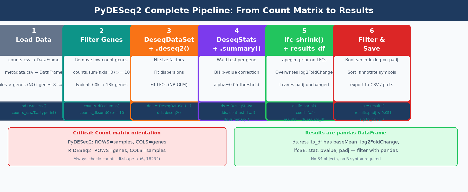
How to Run Differential Expression Analysis with PyDESeq2

The PyDESeq2 workflow separates into two steps: DeseqDataSet for model fitting, DeseqStats for hypothesis testing.

Step 1: Fit the Model with DeseqDataSet

from pydeseq2.dds import DeseqDataSet
from pydeseq2.default_inference import DefaultInference

# DefaultInference controls parallelization
inference = DefaultInference(n_cpus=8)

# Create and fit the DeseqDataSet
dds = DeseqDataSet(
    counts     = counts_df,
    metadata   = metadata,
    design     = "~condition",      # statistical design formula
    refit_cooks = True,             # refit genes with Cook's distance outliers
    inference  = inference
)

# Fit the model: estimates size factors, dispersions, and LFCs
dds.deseq2()

The dds.deseq2() call runs three steps and prints progress for each:

Fitting size factors...
...done in 0.02 seconds.
Fitting dispersions...
...done in 4.31 seconds.
Fitting LFCs...
...done in 3.87 seconds.
Replacing 2 outliers.
Refitting 2 outliers.
...done in 0.14 seconds.

Size factors are accessible at dds.obsm["size_factors"]. Dispersion estimates are in dds.varm["dispersions"]. You can plot the dispersion curve:

dds.plot_dispersions()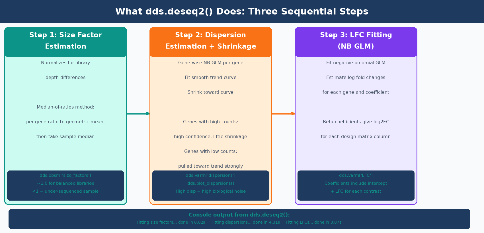

Three-panel diagram showing the three steps inside dds.deseq2(): left panel shows size factor estimation with per-sample bar chart, center panel shows dispersion estimation with gene-wise estimates and fitted trend curve, right panel shows LFC fitting with coefficient estimates per gene — Figure 2: The three steps inside dds.deseq2(). Size factors normalize library depth. Dispersion estimation uses information across all genes to produce stable per-gene estimates. LFC fitting produces the fold change estimates that DeseqStats will test.

Step 2: Run Statistical Tests with DeseqStats

from pydeseq2.ds import DeseqStats

# Create DeseqStats object with a contrast
# contrast = ["variable", "tested_level", "reference_level"]
ds = DeseqStats(
    dds,
    contrast            = ["condition", "treated", "control"],
    alpha               = 0.05,   # significance threshold for summary()
    cooks_filter        = True,   # filter genes with Cook's outliers
    independent_filter  = True,   # independent filtering to improve power
    inference           = inference
)

# Run the Wald test and BH multiple testing correction
ds.summary()

ds.summary() prints:

Running Wald tests...
...done in 2.14 seconds.
Log2 fold change & Wald test p-value: condition treated vs control

          baseMean  log2FoldChange     lfcSE       stat      pvalue        padj
BRCA1    1247.302         -1.432     0.124     -11.558   5.42e-31   1.13e-27
MYC      3890.441          2.891     0.089      32.483   1.21e-231  2.51e-227
...

Number of genes with padj < 0.05:  1842

The results are now in ds.results_df, a standard pandas DataFrame.

How to Apply LFC Shrinkage in PyDESeq2

Like DESeq2 in R, the log2FoldChange column in ds.results_df before shrinkage contains MLE estimates that are noisy for lowly expressed genes. Apply lfc_shrink() to produce apeglm-shrunken estimates for visualization and ranking:

# Apply apeglm LFC shrinkage
# The coeff argument specifies which model coefficient to shrink
ds.lfc_shrink(coeff="condition_treated_vs_control")

# lfc_shrink() overwrites ds.results_df in place
# Verify shrinkage was applied:
print(ds.shrunk_LFCs)  # True

Important: In PyDESeq2, lfc_shrink() modifies ds.results_df in place, overwriting the log2FoldChange column. If you need to compare shrunk and unshrunk values, save the unshrunk DataFrame before calling lfc_shrink():

# Save unshrunk results before shrinkage
results_unshrunk = ds.results_df.copy()

# Apply shrinkage (modifies ds.results_df in place)
ds.lfc_shrink(coeff="condition_treated_vs_control")

# Now ds.results_df contains shrunk LFCs
results_shrunk = ds.results_df.copy()

# Compare a few genes
print(results_unshrunk[["log2FoldChange"]].head())
print(results_shrunk[["log2FoldChange"]].head())

lfc_shrink() changes log2FoldChange but not padj

Like in R, apeglm shrinkage in PyDESeq2 modifies only the log2FoldChange and lfcSE columns. The pvalue and padj columns remain unchanged. Use the shrunk DataFrame for volcano plots, MA plots, and GSEA input. Report significance based on padj regardless of whether shrinkage was applied.

How to Filter and Save PyDESeq2 Results

Since ds.results_df is a pandas DataFrame, filtering and saving uses standard pandas operations:

# Access the results DataFrame
results = ds.results_df.copy()

print(f"Total genes in results: {len(results)}")
print(f"Genes with NA padj (filtered by DESeq2): {results['padj'].isna().sum()}")

# Filter to significant DEGs
sig_degs = results[
    (results["padj"] < 0.05) &
    (results["log2FoldChange"].abs() > 1.0)  # 2-fold change
].copy()

print(f"Significant DEGs (padj<0.05, |LFC|>1): {len(sig_degs)}")
print(f"  Upregulated:   {(sig_degs['log2FoldChange'] > 0).sum()}")
print(f"  Downregulated: {(sig_degs['log2FoldChange'] < 0).sum()}")

# Sort by significance
sig_degs = sig_degs.sort_values("padj")

# Save all genes (for GSEA — needs full ranked list)
results.sort_values("log2FoldChange", ascending=False).to_csv(
    "results/pydeseq2_all_genes_ranked.csv"
)

# Save significant DEGs
sig_degs.to_csv("results/pydeseq2_significant_degs.csv")

print("\nTop 10 significant DEGs:")
print(sig_degs.head(10)[["baseMean", "log2FoldChange", "padj"]])

Adding Gene Symbols to the Results Table

PyDESeq2 results use the same gene IDs as the count matrix columns. If you used Ensembl IDs, map them to symbols using mygene:

import mygene

# Install with: pip install mygene
mg = mygene.MyGeneInfo()

# Strip version numbers from ENSEMBL IDs
gene_ids_clean = [g.split(".")[0] for g in results.index]

# Query gene symbols in bulk (much faster than row-by-row)
gene_info = mg.querymany(
    gene_ids_clean,
    scopes  = "ensembl.gene",
    fields  = "symbol",
    species = "human",
    as_dataframe = True
)

# Map symbols back to results
symbol_map = gene_info["symbol"].drop_duplicates()
results["gene_id"] = gene_ids_clean
results["symbol"]  = results["gene_id"].map(symbol_map)

print(f"Genes with symbol mapping: {results['symbol'].notna().sum()} / {len(results)}")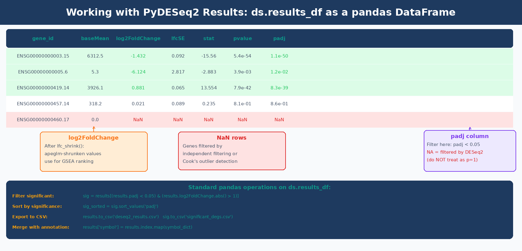

Diagram showing ds.results_df as a pandas DataFrame with columns baseMean, log2FoldChange, lfcSE, stat, pvalue, and padj, with arrows showing pandas operations: .copy() to save before shrinkage, boolean indexing to filter significant genes, .sort_values() to rank, and .to_csv() to save output files — Figure 3: PyDESeq2 results live in a standard pandas DataFrame. The full Python data science toolchain applies directly: boolean indexing for filtering, merge for annotation, to_csv for export, and matplotlib/seaborn for visualization.

Running a Multi-Factor Design in PyDESeq2

Adding a batch variable or additional covariate to the design formula uses the same syntax as R:

# Multi-factor design: control for batch while testing condition
dds_batch = DeseqDataSet(
    counts    = counts_df,
    metadata  = metadata,
    design    = "~batch + condition",  # batch is modeled, condition is tested
    refit_cooks = True,
    inference = inference
)
dds_batch.deseq2()

# Stats: same as before — contrast specifies condition effect
ds_batch = DeseqStats(
    dds_batch,
    contrast   = ["condition", "treated", "control"],
    alpha      = 0.05,
    inference  = inference
)
ds_batch.summary()
ds_batch.lfc_shrink(coeff="condition_treated_vs_control")

results_batch = ds_batch.results_df.copy()

The batch variable absorbs variance attributable to library preparation batches, which increases the power to detect the condition effect. If you know samples were prepared in batches, always include batch in the design.

Running Multiple Contrasts from One Fitted Model

When your experiment has three or more conditions, fit the model once and run multiple contrasts:

# Three-condition experiment: control, dose_low, dose_high
# Assume metadata["condition"] has all three levels

dds_multi = DeseqDataSet(
    counts    = counts_df_multi,
    metadata  = metadata_multi,
    design    = "~condition",
    inference = inference
)
dds_multi.deseq2()

# Run each contrast independently (model fitting is shared)
contrasts_to_run = [
    ("dose_low",  "control"),
    ("dose_high", "control"),
    ("dose_high", "dose_low"),
]

all_results = {}
for tested, ref in contrasts_to_run:
    ds_c = DeseqStats(
        dds_multi,
        contrast  = ["condition", tested, ref],
        alpha     = 0.05,
        inference = inference
    )
    ds_c.summary()
    ds_c.lfc_shrink(coeff=f"condition_{tested}_vs_{ref}")
    all_results[f"{tested}_vs_{ref}"] = ds_c.results_df.copy()
    n_sig = (ds_c.results_df["padj"] < 0.05).sum()
    print(f"{tested} vs {ref}: {n_sig} significant genes")

Generating Visualizations from PyDESeq2 Results

PyDESeq2 includes a built-in MA plot method. For publication-quality plots, use matplotlib or seaborn on ds.results_df directly.

For a plotting deep dive, the same interpretation logic carries into How to Make Volcano Plots and MA Plots in R: ggplot2 and EnhancedVolcano, and the ranked-list follow-up is What Is GSEA and Why Does It Beat a Simple DEG List.

MA Plot

import matplotlib.pyplot as plt
import numpy as np

# Built-in MA plot (requires prior ds.summary() call)
ds.plot_MA(s=5)
plt.title("MA Plot: treated vs control")
plt.savefig("results/ma_plot.pdf", bbox_inches="tight")

Volcano Plot

fig, ax = plt.subplots(figsize=(8, 6))

# Compute -log10(padj), handle NaN
plot_df = results.dropna(subset=["padj", "log2FoldChange"]).copy()
plot_df["neg_log10_padj"] = -np.log10(plot_df["padj"].clip(lower=1e-300))

# Color by significance
is_sig = (plot_df["padj"] < 0.05) & (plot_df["log2FoldChange"].abs() > 1.0)

ax.scatter(
    plot_df.loc[~is_sig, "log2FoldChange"],
    plot_df.loc[~is_sig, "neg_log10_padj"],
    color = "lightgray", s = 5, alpha = 0.7, label = "Not significant"
)
ax.scatter(
    plot_df.loc[is_sig, "log2FoldChange"],
    plot_df.loc[is_sig, "neg_log10_padj"],
    color = "#e63946", s = 8, alpha = 0.8, label = "Significant"
)

ax.axhline(-np.log10(0.05), ls="--", color="gray", lw=1)
ax.axvline( 1.0,            ls="--", color="gray", lw=1)
ax.axvline(-1.0,            ls="--", color="gray", lw=1)

ax.set_xlabel("log2 Fold Change (treated vs control)", fontsize=12)
ax.set_ylabel("-log10(adjusted p-value)", fontsize=12)
ax.set_title("Volcano Plot: treated vs control")
ax.legend(frameon=False)

n_up   = (is_sig & (plot_df["log2FoldChange"] > 0)).sum()
n_down = (is_sig & (plot_df["log2FoldChange"] < 0)).sum()
ax.text(0.98, 0.98, f"Up: {n_up}\nDown: {n_down}",
        transform=ax.transAxes, ha="right", va="top", fontsize=10)

plt.tight_layout()
plt.savefig("results/volcano_plot.pdf", bbox_inches="tight", dpi=150)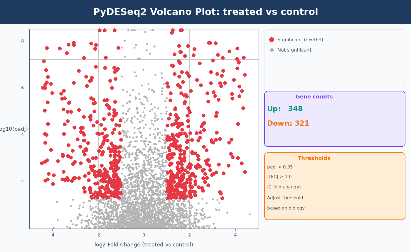

Complete PyDESeq2 Pipeline Script

Here is the full workflow in a single reusable script:

#!/usr/bin/env python3
"""
pydeseq2_pipeline.py

Complete PyDESeq2 differential expression analysis.
Input:  counts.csv  (samples × genes, integer counts)
        metadata.csv (samples × variables)
Output: pydeseq2_results_annotated.csv
        pydeseq2_significant_degs.csv
        volcano_plot.pdf
"""

import pandas as pd
import numpy as np
import matplotlib.pyplot as plt
from pydeseq2.dds import DeseqDataSet
from pydeseq2.default_inference import DefaultInference
from pydeseq2.ds import DeseqStats

# ── 1. Load and validate inputs ──────────────────────────────────
counts_raw = pd.read_csv("results/counts/counts.csv", index_col=0)
counts_df  = counts_raw.T.astype(int)   # transpose: samples × genes

metadata = pd.read_csv("data/sample_metadata.csv",
                        index_col=0,
                        dtype=str)      # keep all columns as strings

assert list(counts_df.index) == list(metadata.index), \
    "Row order mismatch between counts and metadata"

print(f"Samples: {counts_df.shape[0]}   Genes (pre-filter): {counts_df.shape[1]}")

# ── 2. Filter low-count genes ────────────────────────────────────
genes_to_keep = counts_df.columns[counts_df.sum(axis=0) >= 10]
counts_df = counts_df[genes_to_keep]
print(f"Genes (post-filter): {counts_df.shape[1]}")

# ── 3. Fit model ─────────────────────────────────────────────────
inference = DefaultInference(n_cpus=8)

dds = DeseqDataSet(
    counts      = counts_df,
    metadata    = metadata,
    design      = "~condition",
    refit_cooks = True,
    inference   = inference
)
dds.deseq2()

# ── 4. Run statistical test ──────────────────────────────────────
ds = DeseqStats(
    dds,
    contrast   = ["condition", "treated", "control"],
    alpha      = 0.05,
    inference  = inference
)
ds.summary()

# ── 5. Apply LFC shrinkage ───────────────────────────────────────
results_unshrunk = ds.results_df.copy()
ds.lfc_shrink(coeff="condition_treated_vs_control")
results = ds.results_df.copy()

# ── 6. Filter and save ───────────────────────────────────────────
sig = results[
    (results["padj"] < 0.05) &
    (results["log2FoldChange"].abs() > 1.0)
].sort_values("padj")

print(f"\nSignificant DEGs: {len(sig)}")
print(f"  Up: {(sig['log2FoldChange'] > 0).sum()}  "
      f"Down: {(sig['log2FoldChange'] < 0).sum()}")

results.to_csv("results/pydeseq2_all_genes.csv")
sig.to_csv("results/pydeseq2_significant_degs.csv")

# ── 7. Volcano plot ──────────────────────────────────────────────
plot_df = results.dropna(subset=["padj"]).copy()
plot_df["neg_log10_padj"] = -np.log10(plot_df["padj"].clip(lower=1e-300))
is_sig = (plot_df["padj"] < 0.05) & (plot_df["log2FoldChange"].abs() > 1.0)

fig, ax = plt.subplots(figsize=(7, 5))
ax.scatter(plot_df.loc[~is_sig, "log2FoldChange"],
           plot_df.loc[~is_sig, "neg_log10_padj"],
           s=4, color="lightgray", alpha=0.6)
ax.scatter(plot_df.loc[is_sig, "log2FoldChange"],
           plot_df.loc[is_sig, "neg_log10_padj"],
           s=7, color="#e63946", alpha=0.8)
ax.axhline(-np.log10(0.05), ls="--", color="gray", lw=0.8)
ax.axvline(1.0,  ls="--", color="gray", lw=0.8)
ax.axvline(-1.0, ls="--", color="gray", lw=0.8)
ax.set(xlabel="log2 Fold Change", ylabel="-log10(padj)",
       title="PyDESeq2: treated vs control")
plt.tight_layout()
plt.savefig("results/volcano_plot.pdf", dpi=150, bbox_inches="tight")
print("Volcano plot saved.")

NotchBio runs the equivalent of this pipeline internally for Python-based workflows, producing the same normalized counts, Wald test results, and shrunk LFCs in an automated environment. If you prefer to skip the environment setup and get directly to interpreting results, upload your count matrix and metadata at notchbio.app.

Read another related post

View all posts

Research Guide