What Is GSEA and Why Does It Beat a Simple DEG List

You run DESeq2. You get 400 significant genes. You stare at the list. Some of them you recognize — a few metabolism genes, a handful of stress response markers, some things you have never heard of. The biology is in there somewhere, but extracting it from a flat ranked list is slow, subjective, and deeply dependent on how well you happen to know the literature for each gene you are looking at.

This is the problem that Gene Set Enrichment Analysis was designed to solve. Instead of asking “which individual genes changed?”, GSEA asks “do the genes in this known biological pathway tend to be consistently up or down across the full experiment?” The shift from gene-level to pathway-level thinking is not just cosmetic — it is statistically necessary when the real biology is a coordinated modulation of a pathway where each individual gene changes by a small but consistent amount that falls below your significance threshold on its own. If you want the mechanics behind the DE results that usually feed into this step, How DESeq2 Actually Works (Without the Math Overload) is the natural prequel.

The original GSEA paper by Subramanian, Tamayo, Mootha, and colleagues at the Broad Institute was published in PNAS in 2005. They demonstrated the method on muscle biopsies from diabetics versus healthy controls, where genes involved in oxidative phosphorylation showed reduced expression in diabetics — not through large changes in individual genes, but through a coordinated 20% average decrease across the entire pathway. No gene-level cutoff would have caught it. GSEA did (Subramanian et al., PNAS, 2005).

GSEA vs. Over-Representation Analysis: Two Different Questions

Before understanding how GSEA works, it helps to understand what it replaced.

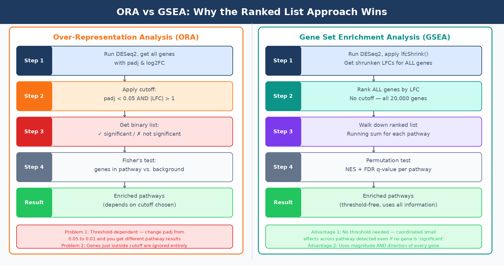
The traditional approach — Over-Representation Analysis (ORA) — starts with your list of significant DEGs (padj < 0.05, say) and asks: is the number of genes from pathway X in this list higher than you would expect by chance? The answer is a Fisher’s exact test or hypergeometric test. It is simple, fast, and widely used.

ORA has two structural problems. First, it throws away continuous information. Every gene in your experiment gets reduced to a binary: significant or not. The gene with padj = 0.001 and a fold change of 4 counts the same as the gene with padj = 0.049 and a fold change of 0.6. The gene with padj = 0.051 — just outside your cutoff — contributes nothing, even if it belongs to a pathway where twenty other members are highly significant.

Second, ORA is sensitive to your significance threshold. Change it from 0.05 to 0.01 and you get a different pathway list. The pathway biology did not change; your arbitrary cutoff did.

GSEA avoids both problems by using all genes, ranked by a continuous metric, without any cutoff. Every gene in your experiment participates in the analysis. The method asks whether a pathway’s members are non-randomly distributed within that full ranked list — whether they tend to pile up at one end rather than scatter uniformly across the whole thing.

The Algorithm Step by Step

GSEA takes two inputs: a ranked gene list and a collection of gene sets.

The ranked gene list is every gene in your experiment, ordered from most upregulated to most downregulated. The ranking metric is usually the shrunken log2 fold change from DESeq2, the signed negative log10 p-value, or the Wald test statistic. All three are common; the signed statistic or shrunken LFC is generally preferred because it captures both effect direction and magnitude. That choice becomes easier to understand once you have seen how DESeq2 estimates shrunken fold changes and how it compares with alternatives like edgeR and limma-voom.

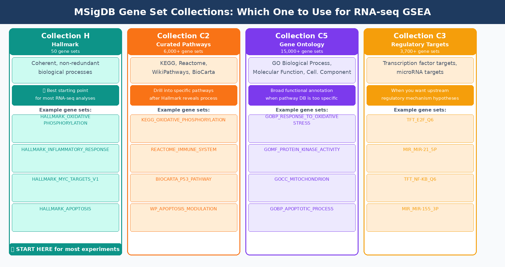
The gene sets are curated collections of genes that share a biological function, pathway membership, chromosomal location, or regulatory relationship. The standard source is the Molecular Signatures Database (MSigDB), maintained by the Broad Institute. MSigDB contains nine collections. For most RNA-seq experiments, three are most useful: the Hallmark collection (H), which contains 50 well-curated gene sets representing coherent biological processes; the Curated Pathways collection (C2), which includes KEGG, Reactome, and WikiPathways; and the Gene Ontology collection (C5).

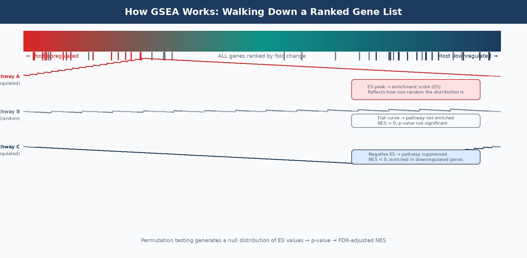
Once you have a ranked list and a gene set, the algorithm works as follows. Walk down the ranked list from top (most upregulated) to bottom (most downregulated). For each gene, increment a running sum if the gene is a member of the pathway being tested, decrement it if the gene is not. The running sum is weighted by how far from the center of the list each gene lands — genes at the extreme top or bottom (high fold change, strong signal) contribute more to the score than genes in the middle.

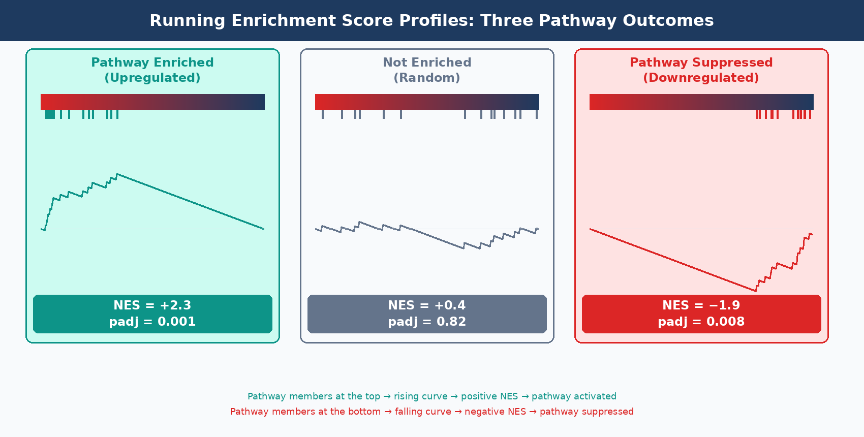
The enrichment score (ES) is the maximum deviation of the running sum from zero. A pathway where all its members are clustered at the top of the ranked list produces a running sum that climbs sharply and peaks high. A pathway whose members are scattered randomly produces a running sum that wanders near zero. The peak position and height encode both which direction the pathway is regulated and how strongly its members are coordinated.

Statistical significance is assessed by permutation. The observed ES is compared to a null distribution generated by randomly permuting either the gene labels or the sample labels thousands of times and recalculating the ES each time. The normalized enrichment score (NES) corrects the ES for gene set size, allowing comparison across pathways of different sizes. The false discovery rate (FDR q-value) adjusts for multiple testing across all gene sets tested.

What the Output Columns Mean

A GSEA results table typically contains these columns. Each has a specific interpretation that differs from what you might assume coming from a DESeq2 results table.

The leading edge subset is one of GSEA’s most underused outputs. These are the genes within the enriched pathway that appear before the peak of the running sum — the genes that actually contribute most to the enrichment score. When a pathway is significantly enriched, the leading edge tells you which specific members are driving it. Two pathways enriched with the same NES can have completely different leading edges, pointing to different biological mechanisms.

A common threshold for GSEA significance is padj < 0.25 rather than the more typical 0.05. The Broad Institute’s original recommendation was to consider gene sets with FDR q-value < 0.25 as candidates for follow-up. This more permissive threshold reflects the fact that GSEA is hypothesis-generating — you are identifying processes worth investigating, not making final claims. For publication-ready results, padj < 0.05 is more defensible and is the default in fgsea.

Running GSEA in R with fgsea

The standard current implementation for R is fgsea, which implements a fast version of pre-ranked GSEA using an adaptive multilevel Monte Carlo scheme. It is substantially faster than the original Broad GSEA and is the backend used by clusterProfiler::GSEA().

library(fgsea)
library(msigdbr)
library(DESeq2)
library(dplyr)

# Step 1: Get DESeq2 shrunken LFC results
res_shrunk <- lfcShrink(dds, coef = "condition_treated_vs_control", type = "apeglm")

# Step 2: Build ranked gene list — shrunken LFC, named by gene symbol
# Remove NAs and sort descending (most upregulated first)
ranked_genes <- res_shrunk %>%
  as.data.frame() %>%
  filter(!is.na(log2FoldChange), !is.na(padj)) %>%
  arrange(desc(log2FoldChange)) %>%
  { setNames(.$log2FoldChange, rownames(.)) }

# Step 3: Get MSigDB Hallmark gene sets for your organism
msigdbr_df <- msigdbr(species = "Homo sapiens", category = "H")
pathways_H  <- split(msigdbr_df$gene_symbol, msigdbr_df$gs_name)

# Step 4: Run fgsea
set.seed(42)  # for reproducibility — fgsea uses Monte Carlo permutations
fgsea_res <- fgsea(
  pathways  = pathways_H,
  stats     = ranked_genes,
  minSize   = 15,   # exclude very small gene sets (unreliable ES)
  maxSize   = 500   # exclude very large gene sets (too broad to interpret)
)

# Step 5: Sort by NES and inspect
fgsea_res_sorted <- fgsea_res %>%
  arrange(desc(NES)) %>%
  filter(padj < 0.05)

head(fgsea_res_sorted[, c("pathway","NES","padj","size","leadingEdge")])

Interpreting GSEA Results: What Enrichment Actually Means

A positive NES means the pathway’s member genes tend to be upregulated in your treatment condition relative to control. A negative NES means they tend to be downregulated. Both can be biologically significant — pathway suppression is as meaningful as pathway activation.

The NES alone does not tell you which individual genes are responsible. That is what the leading edge is for. When you see HALLMARK_OXIDATIVE_PHOSPHORYLATION enriched with NES = −2.1 in your treated samples, the leading edge tells you precisely which components of the oxidative phosphorylation machinery are most suppressed — it might be Complex I subunits, or electron transport chain genes, or ATP synthase components. That specificity transforms a pathway-level observation into a mechanistic hypothesis.

When multiple gene sets are enriched, look at their leading edge overlap. Two pathways with 80% of the same leading edge genes are detecting the same underlying biological signal. This is common in MSigDB C2, where many curated pathways share genes. The Hallmark collection was built specifically to reduce this redundancy — which is why it is the better starting point.

Common Mistakes and How to Avoid Them

Using a cutoff to pre-filter genes before GSEA. GSEA is designed to use all genes ranked by a continuous metric. Filtering to significant DEGs before ranking defeats the purpose of the method — you are reintroducing the binary cutoff problem that GSEA was designed to avoid. Feed the full ranked list, not just significant genes.

Using raw p-values as the ranking metric without directional information. Ranking by p-value alone lumps upregulated and downregulated genes at the same end of the list (both have low p-values). The result is that pathways enriched in upregulated genes and pathways enriched in downregulated genes get mixed together. The recommended ranking metric is signed statistic: sign(log2FoldChange) * -log10(pvalue), or simply the shrunken LFC. Both preserve directionality.

Running GSEA with very small gene sets (fewer than 15 genes). The enrichment score for a small gene set is highly variable — a single outlier gene can dominate the ES. The minSize = 15 parameter in fgsea removes these unreliable tests. The maxSize = 500 parameter removes gene sets so large that they are not interpretable as discrete pathways.

Interpreting NES magnitude across different gene set databases. NES is normalized within a database and run, so you cannot compare the NES of a Hallmark result to the NES from a C2 result from a different run. Use NES to rank within one GSEA run on one database.

Forgetting to set a seed. fgsea uses Monte Carlo permutations. Results will differ slightly between runs without a fixed seed. For reproducibility in any published analysis, always call set.seed() before fgsea().

When GSEA Is the Right Tool, and When It Is Not

GSEA works best when your experiment has a clear phenotypic contrast — treated versus control, disease versus healthy — and when you have reasonable sample sizes (at least three replicates, ideally more). The permutation-based statistics are more reliable with more samples.

GSEA is less appropriate when your experiment has very few replicates, your signal is very noisy (many genes near padj = 1.0), or you are exploring single-cell data where pseudobulk approaches are necessary before pathway analysis. For single-cell data, the recommended path is pseudobulk aggregation per sample per cell type, followed by DESeq2 and then GSEA on the pseudobulk results.

GSEA is also not the right tool for the question “which specific genes are different?” That is still a DEG list question. GSEA answers “which processes are coordinated across the experiment?” The two questions are complementary and most analysis pipelines include both.

NotchBio runs fgsea against the MSigDB Hallmark collection automatically after every DESeq2 analysis, and makes the full NES-ranked results table — including leading edge genes for every enriched pathway — available in the results dashboard. You can swap in C2 or C5 collections and re-run without touching any code. If you want pathway-level biology from your RNA-seq data without configuring clusterProfiler manually, start at notchbio.app.