When to Use edgeR vs DESeq2 vs limma-voom
There is a version of this question that gets asked constantly in bioinformatics forums: which tool is best for differential expression? The answer that people want is a clean ranking. The answer that is actually true is more useful: they solve the same problem using different statistical machinery, and each one has specific scenarios where it genuinely outperforms the others.
DESeq2 and edgeR both model counts using the negative binomial distribution. limma-voom transforms counts into continuous values and applies linear models with empirical Bayes moderation originally developed for microarrays. That difference in statistical philosophy flows through to every aspect of how they behave — what they find, what they miss, how conservative they are, and which experimental designs they handle gracefully.
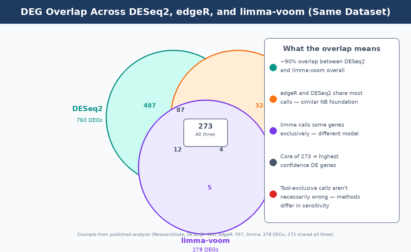
The overlap between what all three tools call significant is high. A published analysis detected 760 significant DEGs with DESeq2, 597 with edgeR, and 278 with limma-voom, with 273 genes overlapping across all three (ResearchGate). Broader benchmarks consistently show around 90% overlap between DESeq2 and limma-voom results. What differs is who calls that remaining 10%, and whether those calls are true positives or false alarms.
This post explains the statistical machinery behind each tool, where each one has a genuine advantage, and how to make the call for your specific experiment. If you want a deeper look at just one of these frameworks before comparing all three, How DESeq2 Actually Works (Without the Math Overload) is the best place to start. If your model choice is being driven by technical confounding, Batch Effects: The Silent Killer of RNA-Seq Studies is the companion post.
The Shared Foundation and Where the Tools Diverge
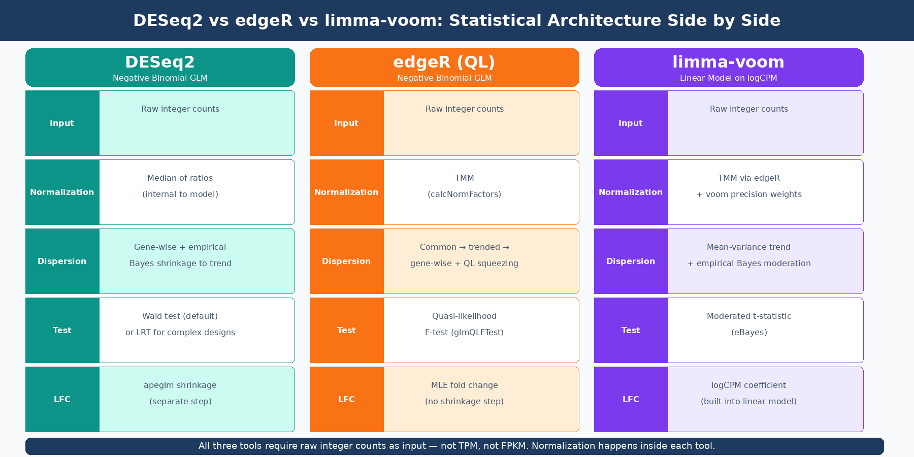
All three tools start from a raw count matrix and end with a ranked list of genes accompanied by fold changes and adjusted p-values. The divergence is in the middle: how they model the data, how they estimate variance, and what statistical test they ultimately apply.
DESeq2 fits a negative binomial generalized linear model per gene. Normalization is done via the median of ratios method, internal to the model itself. The key innovation is its empirical Bayes shrinkage of dispersion estimates toward a gene-expression-trend prior, which makes it robust when replicate counts are low. The Wald test is the default for simple pairwise comparisons; the likelihood ratio test is available for complex multi-factor designs. As covered in the DESeq2 post, size factors and dispersions are estimated as model parameters rather than preprocessing steps, which is why raw integer counts are mandatory as input.
edgeR also uses the negative binomial distribution, but its dispersion estimation strategy differs from DESeq2’s. edgeR estimates a common dispersion across all genes, then trended and gene-specific dispersions, and uses a weighted likelihood approach to combine them. Normalization uses TMM (Trimmed Mean of M-values), which edgeR pioneered and which is now the default normalization in limma as well. edgeR offers two testing frameworks: the classic exact test (best for simple two-group comparisons) and the quasi-likelihood (QL) F-test (better for complex designs because it more conservatively handles variability in dispersion estimates across genes).
limma-voom takes a fundamentally different approach. The voom function transforms raw counts to log2-counts-per-million (logCPM) and, critically, estimates the mean-variance relationship of those logCPM values to compute precision weights for each observation. Those weights capture the fact that low-count observations carry more uncertainty. The precision-weighted logCPM values are then fed into limma’s linear modeling framework, which applies empirical Bayes moderation of variance estimates across genes. The result is a moderated t-statistic that borrows information across all genes — the same philosophy as DESeq2’s dispersion shrinkage, but operating in log-space on a continuous transformed variable rather than in count space on integers. A linear model is used for statistics in limma, while the negative binomial distribution is used in edgeR and DESeq2 (PubMed 34605806).
Sensitivity, False Discovery, and What the Benchmarks Say
The clearest difference between the tools in practice is sensitivity versus specificity tradeoff. DESeq2 and edgeR consistently detect more differentially expressed genes than limma-voom, particularly among lowly expressed genes. But comparative studies have shown that DESeq2 and edgeR have inflated false discovery rates in some settings, while limma-voom does not demonstrate excessive false positives (ResearchGate).
This pattern is not a flaw in either approach — it is a consequence of their distributional assumptions. DESeq2 and edgeR model counts directly with a parametric negative binomial model. When those assumptions hold well (which they do for most standard bulk RNA-seq experiments), the sensitivity gain is real. When the data has unusual outliers or the negative binomial is a poor fit, the extra detections can include false positives that limma-voom’s more conservative linear framework avoids.
From the STARTbio comparison: limma-voom calls a substantial number of genes not called by DESeq2 or edgeR. This is partly attributable to limma’s different (Gaussian-based) modeling approach, which captures different projections of the biological variance. That 10% of limma-exclusive calls is not simply wrong — it may reflect real signal that the other two tools are underpowered to detect, particularly at subtle effect sizes (STARTbio).
The practical upshot: if you are trying to maximize sensitivity and are willing to follow up with validation, DESeq2 or edgeR will give you the longest list. If you need conservative, well-controlled FDR — for instance, in a clinical study where false positives are costly — limma-voom is frequently cited as the more disciplined option.
When DESeq2 Is the Right Default
DESeq2 is the appropriate default for most standard bulk RNA-seq experiments: two conditions, three to six biological replicates, human or model organism data, routine two-group comparison.
Its dispersion shrinkage makes it particularly well-calibrated for small sample sizes. With three replicates per group, per-gene dispersion estimates are unreliable. DESeq2’s empirical Bayes approach borrows strength across thousands of genes to produce more reliable estimates than you could get from three data points alone. edgeR’s quasi-likelihood model does something similar, but DESeq2’s implementation is generally considered more conservative and better-calibrated in the very small sample regime.
DESeq2’s batch effect handling via the design formula (~ batch + condition) is clean and well-documented, and its independence filtering and Cook’s distance outlier detection are automatic safeguards that edgeR does not apply by default.
Concretely: if you are running a treatment-versus-control experiment with three replicates per arm, starting from raw STAR or featureCounts output, DESeq2 is where most practitioners begin and where most stay. Downstream, those same DESeq2 results are often used to power pathway analysis with GSEA, which is one reason stable fold change estimation matters.
library(DESeq2)
dds <- DESeqDataSetFromMatrix(  countData = count_matrix,  colData   = metadata,          # must include 'condition' column  design    = ~ condition)
dds <- DESeq(dds)res <- results(dds, contrast = c("condition", "treated", "control"))res_shrunk <- lfcShrink(dds, coef = "condition_treated_vs_control", type = "apeglm")
When edgeR Has the Edge
edgeR’s primary advantage is its handling of very low count genes and its flexibility in normalization. The original developers note that edgeR is generally preferred for applications with lots of small counts (Bioconductor support, 2026).
With the quasi-likelihood framework introduced in edgeR v3 (and further refined in edgeR v4), edgeR handles overdispersion more conservatively than the classic exact test. The QL F-test, now the recommended default workflow, provides better type I error control in datasets where gene-wise dispersions vary substantially from the global trend.
edgeR also has a natural computational advantage for large datasets. In benchmarks, edgeR and limma ran in seconds on datasets where DESeq2 took minutes (PMC4293378). For analyses that need to be run iteratively (many contrasts, many subsets, or multi-tissue comparisons), this speed difference becomes material.
The edgeR workflow for a simple pairwise comparison:
library(edgeR)
# DGEList creation and TMM normalizationdge <- DGEList(counts = count_matrix, group = metadata$condition)dge <- calcNormFactors(dge, method = "TMM")
# Design matrixdesign <- model.matrix(~ condition, data = metadata)
# Dispersion estimation (quasi-likelihood framework)dge <- estimateDisp(dge, design)fit <- glmQLFit(dge, design)
# Test: treated vs controlqlf <- glmQLFTest(fit, coef = "conditiontreated")topTags(qlf, n = 20)
Use edgeR's quasi-likelihood F-test rather than the classic exact test
The classic exactTest in edgeR is only appropriate for simple two-group comparisons with no covariates. For any design with batch effects, paired samples, or multiple factors, use glmQLFit + glmQLFTest. The QL F-test has better type I error control than the classic approach and is the current recommended default in edgeR documentation.
When limma-voom Is the Better Choice
limma-voom shines in three specific scenarios: large sample sizes, complex experimental designs, and when you need the full flexibility of linear model contrasts.
Large datasets. As sample sizes grow above 20 or 30 per condition, the negative binomial assumption becomes less critical — large samples provide enough information for each gene to estimate its own variance reliably, and the CLT pushes count distributions toward approximate normality. At that scale, limma-voom’s linear framework performs comparably to DESeq2 and edgeR in sensitivity, while being considerably faster. The voom precision weights ensure that the heteroscedasticity of count data is accounted for even in the linear model framework.
Complex designs. limma’s linear model framework handles arbitrary experimental designs more naturally than DESeq2 or edgeR. Time-series experiments with multiple time points, factorial designs with interaction terms, and experiments with blocking factors (donors, litters, paired samples) map cleanly onto limma’s makeContrasts system. The same model can simultaneously estimate and test dozens of contrasts without re-fitting. edgeR’s GLM framework can handle these designs too, but the contrast specification syntax is more cumbersome for highly factorial designs.
Random effects and nesting. When samples have hierarchical structure — multiple measurements per donor, multiple tissues per animal, matched pairs — limma’s duplicateCorrelation function estimates and accounts for the within-subject correlation, effectively implementing a linear mixed model. This is the recommended approach from the edgeR/limma developers themselves: limma for complex designs with random effects and outlier samples (Bioconductor support, 2026).
The limma-voom workflow:
library(limma)library(edgeR)
# Create DGEList and normalize with TMM (recommended even for limma)dge <- DGEList(counts = count_matrix)dge <- calcNormFactors(dge, method = "TMM")
# Design matrix — works for simple or arbitrarily complex designsdesign <- model.matrix(~ 0 + condition + batch, data = metadata)
# Voom transformation: converts counts to precision-weighted logCPMv <- voom(dge, design, plot = TRUE)
# Linear model fit with empirical Bayes moderationfit  <- lmFit(v, design)contr <- makeContrasts(treated - control, levels = design)fit2  <- contrasts.fit(fit, contr)fit2  <- eBayes(fit2)
topTable(fit2, adjust = "BH", n = 20)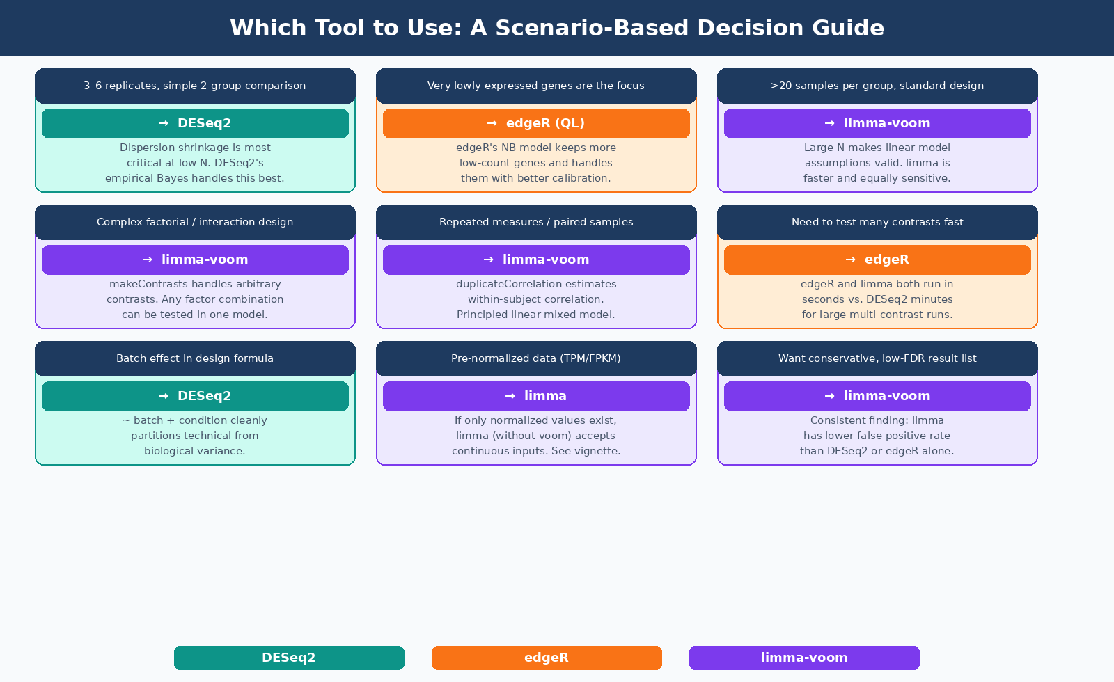
The Overlap Question: Should You Run All Three?
Researchers sometimes run all three tools and report only the genes called significant by two out of three or all three. This approach reduces false positives at the cost of sensitivity — you will miss real DE genes that only one tool detects, but what remains is a highly confident list.
The practical problem is that it is not principled. You are not running a formal consensus test; you are using agreement as a proxy for confidence without a statistical framework for doing so. The intersection is more conservative than any single tool’s adjusted p-value threshold, but by an unknown amount.
A more defensible approach is to pick the tool most appropriate for your design and sample size, apply it once, and use a stringent padj threshold (0.05 with apeglm-shrunken fold changes for DESeq2, or 0.01 if you want extra stringency). If you want to validate robustness, run a second tool as a sensitivity check and note concordance in your methods, but base your biological conclusions on a single primary analysis.
| Criterion | DESeq2 | edgeR (QL) | limma-voom |
|---|---|---|---|
| Statistical model | Negative binomial GLM | Negative binomial GLM | Linear model on logCPM |
| Normalization | Median of ratios (internal) | TMM | TMM (via edgeR) |
| Best sample size | 3–20 per group | 3–10 per group | ≥10 per group |
| Handles low counts | Very good | Excellent | Good |
| Complex designs | Good | Good | Excellent |
| Random effects / paired | Moderate | Moderate | Excellent |
| Sensitivity (DEG count) | High | High | Moderate |
| False positive control | Good | Good | Very good |
| Speed | Moderate | Fast | Fast |
| Input required | Raw integer counts | Raw integer counts | Raw integer counts |
All three tools require raw integer counts as input
Regardless of which tool you choose, the input must be a raw count matrix with integer values — not TPM, not FPKM, not normalized counts. Each tool applies its own normalization internally. Feeding pre-normalized values into any of these tools produces invalid results.
The Practical Decision
For most bulk RNA-seq experiments with three to six replicates and a straightforward two-group or multi-group design: start with DESeq2. It is well-documented, well-validated, and handles the most common edge cases gracefully with built-in safeguards.
If your experiment involves very lowly expressed genes as primary targets, you need to process many contrasts rapidly, or you have limited computational patience: edgeR’s quasi-likelihood framework is an equally rigorous alternative that runs considerably faster.
If your design involves multiple time points, blocking by donor, repeated measurements, or any structure that maps naturally to a linear mixed model: limma-voom, with duplicateCorrelation where applicable, is the more principled choice and the one the tools’ own developers recommend for these scenarios.
All three are published, peer-reviewed, and widely cited. The difference between them, for most standard experiments, is smaller than the variation introduced by differences in alignment strategy, annotation version, or filtering choices. The tool is one decision. Make it deliberately, document it, and move on to the biology.
NotchBio runs DESeq2 by default and exposes edgeR and limma-voom as configurable alternatives in the pipeline settings. All three are available with their current recommended parameter defaults, and the results table is formatted identically regardless of which tool you use. If you want to run all three and compare, that is a built-in option. You can start at notchbio.app.
Further reading
Read another related post
How to Run FastQC and MultiQC on Raw RNA-Seq Reads
A hands-on guide to automating RNA-seq QC across dozens of samples using FastQC and MultiQC, with bash and Python scripts for parsing and flagging failures.
Research GuideRaw Reads to Counts: The Bulk RNA-Seq Pipeline Explained
A practical breakdown of every computational step in bulk RNA-seq: from FASTQ quality control through trimming, alignment, and quantification to your final count matrix.
Research GuideBatch Effects Will Ruin Your RNA-Seq Results
Batch effects silently corrupt bulk RNA-seq data. Learn how to detect them, why they happen, and which correction methods actually work.