Batch Effects: The Silent Killer of RNA-Seq Studies
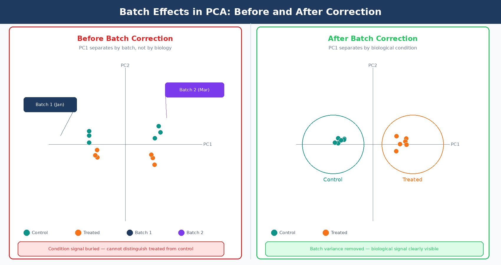
Your PCA plot separates perfectly. Two tight clusters, treatment on the right, control on the left. You feel good about the data. Then someone asks: when were the control samples processed? You check the metadata. Controls: January. Treatment samples: March. Two different RNA extractions, two different library prep kits, two different sequencing runs, two months apart. The clean separation you just called a biological signal is almost certainly a batch effect.
This happens constantly in RNA-seq. Batch effects are systematic, non-biological differences between groups of samples that arise from technical factors during collection, extraction, library preparation, or sequencing. They are not noise in the statistical sense. They are structure: organized, reproducible signals that look exactly like biology until you notice the confound. When they are ignored, they inflate your DE gene list with technical artifacts. When they are overcorrected, they remove real biological signal. Getting this right matters.
This post covers what batch effects are, where they come from, how to detect them before they damage your analysis, and when to use each of the three main correction strategies available to bulk RNA-seq researchers. If the confounding problem itself feels familiar, Experimental Design Mistakes That Kill Your Differential Expression Analysis is the companion piece. If you want the model-level details behind the ~ batch + condition formula, How DESeq2 Actually Works (Without the Math Overload) fills that in.
Where Batch Effects Come From
A batch effect can arise from any technical factor that differs systematically between subsets of samples. The most common sources in bulk RNA-seq are:
Library preparation date or operator. RNA-seq libraries are sensitive to small changes in incubation times, reagent temperatures, and handling technique. Samples prepared on different days, or by different people, accumulate these micro-variations into a measurable systematic signal.
Reagent lot. A new lot of the same kit can have subtly different enzyme activity, buffer pH, or adapter ligation efficiency. Labs that reorder supplies between experiments routinely introduce batch effects without realizing it.
Sequencing platform or run. Samples run on different Illumina instruments, across different flow cells, or on different sequencing dates will carry instrument-specific technical signatures. Even samples from the same instrument but run on different days can differ due to cluster density variations.
RNA integrity differences between processing waves. If half your samples were extracted immediately after tissue collection and the other half were stored at −80°C for six months, they will not be directly comparable even if the RIN scores look acceptable.
Facility or sequencing center. Multi-site studies are particularly susceptible. Different core facilities use different protocols, different alignment pipelines, and sometimes different reference genome versions.
The defining property of a batch effect is that the technical variable is correlated with a group of samples, not distributed randomly across all samples. A single outlier sample is a quality control problem. A pattern where all control samples cluster away from all treatment samples for a documented technical reason is a batch effect.
Batch effects on the scale of biological signal are common, not rare
A widely cited review noted that batch effects can be on a similar scale or even larger than the biological differences of interest, significantly reducing statistical power to detect differentially expressed genes. This is not a niche problem. It is the default state of multi-batch experiments when batches are not carefully designed.
Detecting Batch Effects: What to Look For
Detection is always the first step, and it has to happen before correction. You cannot correct a batch effect you have not confirmed exists, and you definitely cannot correct one that is fully confounded with your biological condition.
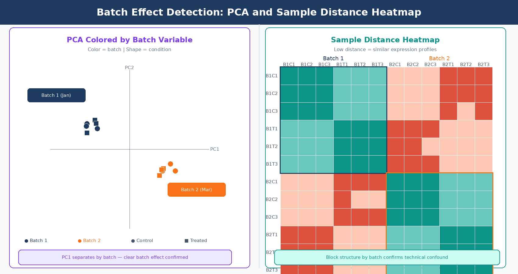
PCA is the primary detection tool. Run a PCA on variance-stabilized counts (VST from DESeq2 is the standard input) and color the points by two things: biological condition and suspected batch variable. If your samples cluster more tightly by batch than by condition in the first two principal components, you have a detectable batch effect.
The pattern to look for is PC1 separating by batch rather than by condition, or large jumps in inter-sample distance between samples from different processing dates that should be biological replicates. Replicates from the same condition should cluster tightly. If they do not, and the spread correlates with a technical variable, that is your signal.
Sample-to-sample distance heatmaps complement PCA by showing pairwise relationships. In a well-designed experiment without batch effects, samples from the same condition cluster in the heatmap. Anomalous clustering by batch date or preparation group is immediately visible.
Hierarchical clustering of samples by expression profile follows the same logic. Dendrogram branches that split by processing date rather than biology indicate a batch effect.
One important caution: PCA visually separates by the largest sources of variance. If your biological effect is large, it will dominate PC1 even in the presence of a batch effect. The batch effect may be pushing PC2 or PC3. Always check more than the first two components, and always color by every technical variable in your metadata, not just the one you suspect most.
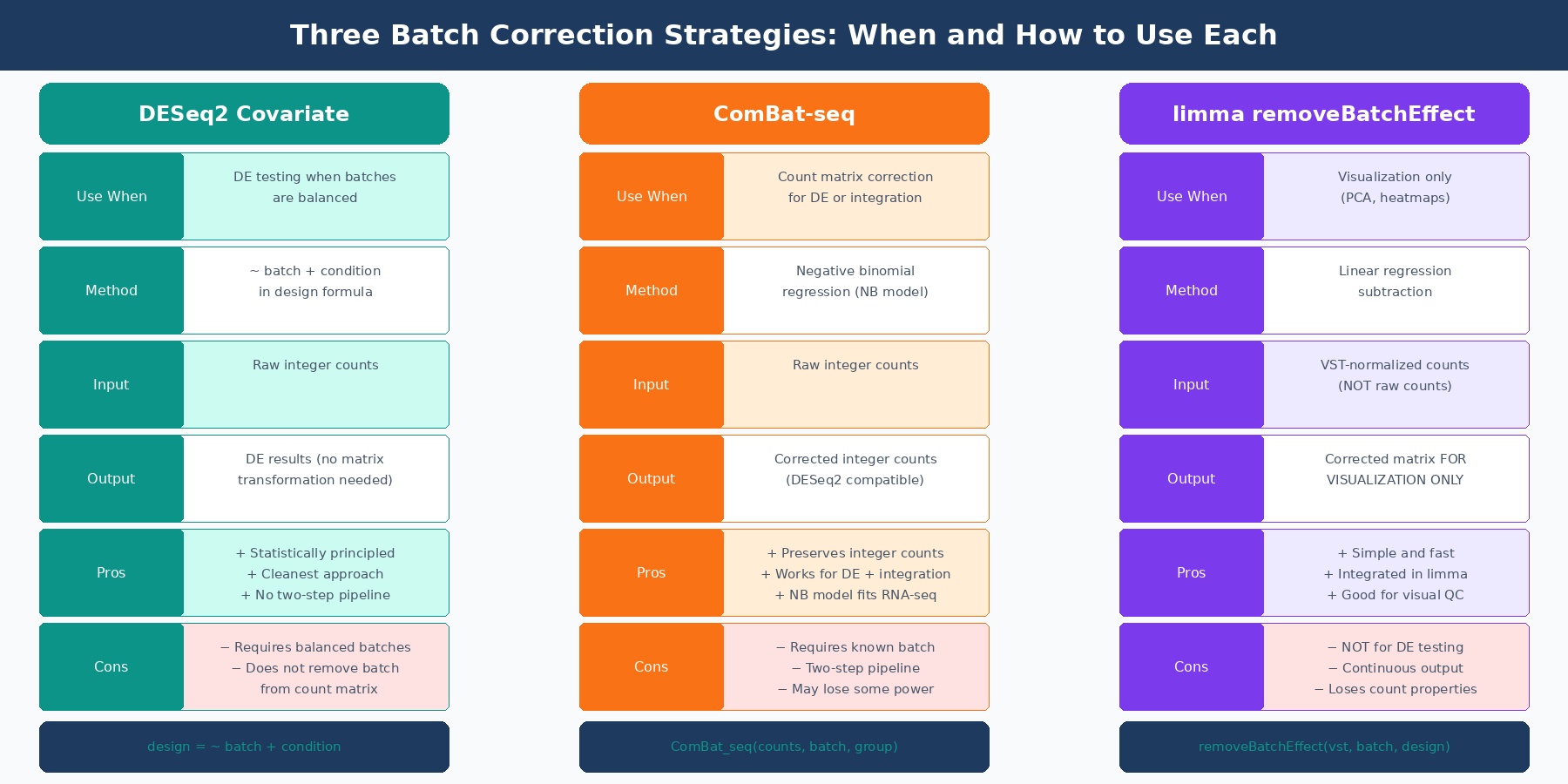
Strategy 1: Include Batch as a Covariate in DESeq2
When batches are balanced across conditions (meaning each batch contains samples from all biological conditions), the cleanest approach is to include batch as a covariate in your DESeq2 design formula and run the differential expression analysis once:
library(DESeq2)
# Load your count matrix and metadatadds <- DESeqDataSetFromMatrix(  countData = count_matrix,  colData   = sample_metadata,   # must contain 'batch' and 'condition' columns  design    = ~ batch + condition # batch listed first, condition is the test factor)
# Run DESeq2 — batch variance is partitioned away automaticallydds <- DESeq(dds)
# Extract results for condition contrastres <- results(dds, contrast = c("condition", "treated", "control"))res_ordered <- res[order(res$padj), ]
This approach is statistically principled and computationally clean. DESeq2 estimates the batch effect as a parameter in its generalized linear model and removes it from the treatment effect estimate. The result is a fold change and adjusted p-value that reflects only the biological contrast of interest.
The critical requirement is balance. If batch and condition are confounded (all controls in batch 1, all treated in batch 2), the batch and condition terms will compete for the same variance and your estimates will be unreliable. DESeq2 will not refuse to run, but the results will be wrong. This is the confounding problem from Experimental Design Mistakes That Kill Your Differential Expression Analysis: it cannot be fixed computationally after the fact.
List batch before condition in your DESeq2 design formula
The order of terms in a DESeq2 design formula matters for which variable is considered first when partitioning variance. Placing batch before condition (~ batch + condition) ensures that known technical variance is accounted for before the biological comparison is tested. The last term in the formula is the one whose effect will be reported in your results.
Strategy 2: ComBat-seq for Count Data Correction
When you need to remove batch effects from the count matrix itself, rather than just model them away, the modern tool for bulk RNA-seq is ComBat-seq (Zhang, Parmigiani, and Johnson, NAR Genomics and Bioinformatics, 2020).
The original ComBat, designed for microarray data, assumes expression values follow a Gaussian distribution. RNA-seq count data is skewed and overdispersed, so the Gaussian assumption fails: applying Gaussian-based correction to count data can produce negative values in the adjusted matrix and generate erroneous significant differences between samples that should be equivalent. ComBat-seq addresses this by using a negative binomial regression model, which correctly models the distributional properties of RNA-seq counts. The critical practical advantage is that ComBat-seq output retains the integer count nature of the data, making the corrected matrix directly compatible with DESeq2 and edgeR without any additional transformation.
library(sva)  # ComBat-seq is in the sva Bioconductor package
# count_matrix: genes × samples integer matrix# batch_vector: factor or integer vector indicating batch for each sample# condition_vector: biological condition (passed as group to preserve biological signal)
adjusted_counts <- ComBat_seq(  counts    = count_matrix,  batch     = batch_vector,  group     = condition_vector,  # preserve biological signal during correction  full_rank = FALSE)
# adjusted_counts is still an integer matrix — safe to pass to DESeq2dds_corrected <- DESeqDataSetFromMatrix(  countData = adjusted_counts,  colData   = sample_metadata,  design    = ~ condition  # batch is now removed, no longer in design)
dds_corrected <- DESeq(dds_corrected)res_corrected <- results(dds_corrected, contrast = c("condition", "treated", "control"))
Passing the group argument is important. Without it, ComBat-seq does not know which variance is biological and may inadvertently correct away the treatment signal along with the batch signal. Always provide the biological grouping variable when you know it.
ComBat-seq is the right tool when you need a corrected count matrix as output: for visualization, for integration with external datasets, for sending corrected data to collaborators, or when running multiple downstream analyses where you want batch-free counts as the starting point.
Strategy 3: limma removeBatchEffect for Visualization
limma::removeBatchEffect is not a differential expression preprocessing tool. It is a visualization tool. The distinction matters.
removeBatchEffect adjusts a normalized expression matrix (typically VST counts from DESeq2) by regressing out the batch variable. The resulting matrix is appropriate for PCA plots, heatmaps, and other visual quality checks where you want to see biological structure unobscured by technical variation. It is explicitly not intended as input for differential expression testing.
library(limma)library(DESeq2)
# Variance-stabilize counts firstvsd <- vst(dds, blind = FALSE)
# Remove batch effect from the VST matrix FOR VISUALIZATION ONLYvsd_corrected <- assay(vsd)vsd_corrected <- removeBatchEffect(  vsd_corrected,  batch   = sample_metadata$batch,  design  = model.matrix(~ condition, data = sample_metadata)  # preserve biological signal)
# Use vsd_corrected for PCA and heatmaps# Do NOT use it as input to DESeq2 or edgeRplotPCA_corrected <- prcomp(t(vsd_corrected))
The design argument in removeBatchEffect serves the same purpose as the group argument in ComBat-seq: it tells the function which variance to preserve rather than remove. Without it, you risk correcting away your biological signal, leaving a matrix where treated and control samples look indistinguishable.
When Correction Is Impossible
All three strategies fail in the same scenario: complete confounding. If every sample in condition A was processed in batch 1 and every sample in condition B was processed in batch 2, there is no statistical way to separate the biological effect from the technical effect. They are one signal. No tool removes this, because the tool cannot know which variance belongs to biology and which belongs to batch when the two are perfectly correlated.
This is worth repeating clearly: batch correction methods, no matter how sophisticated, cannot correct a fully confounded design. The original ComBat-seq paper states this explicitly: “batch correction in confounded designs is challenging for most if not all the state-of-the-art batch adjustment methods, and careful experimental design has been widely advised to mitigate the unfavorable impact of batch effects” (NAR Genomics and Bioinformatics, 2020).
The practical implication is that the most important batch-related decision in an RNA-seq experiment is not which correction tool to use. It is whether to include all conditions in every processing batch at the design stage, before a single sample is collected. A partially confounded design, where at least some samples from each condition appear in each batch, can be corrected. A fully confounded design cannot.
| Situation | Detectable? | Correctable? | Recommended Action |
|---|---|---|---|
| Balanced batches (all conditions in each batch) | Yes (PCA) | Yes | Include as covariate in DESeq2 design |
| Partially confounded (some overlap) | Yes (PCA) | Partially | ComBat-seq or DESeq2 covariate with caution |
| Fully confounded (batch = condition) | Yes (PCA) | No | Redo the experiment with balanced design |
| Unknown batch (no metadata) | Sometimes (SVA) | Partially | Use surrogate variable analysis (SVA) |
| Batch effect smaller than biological signal | May be masked | Not needed | Model if known, ignore if not detectable |
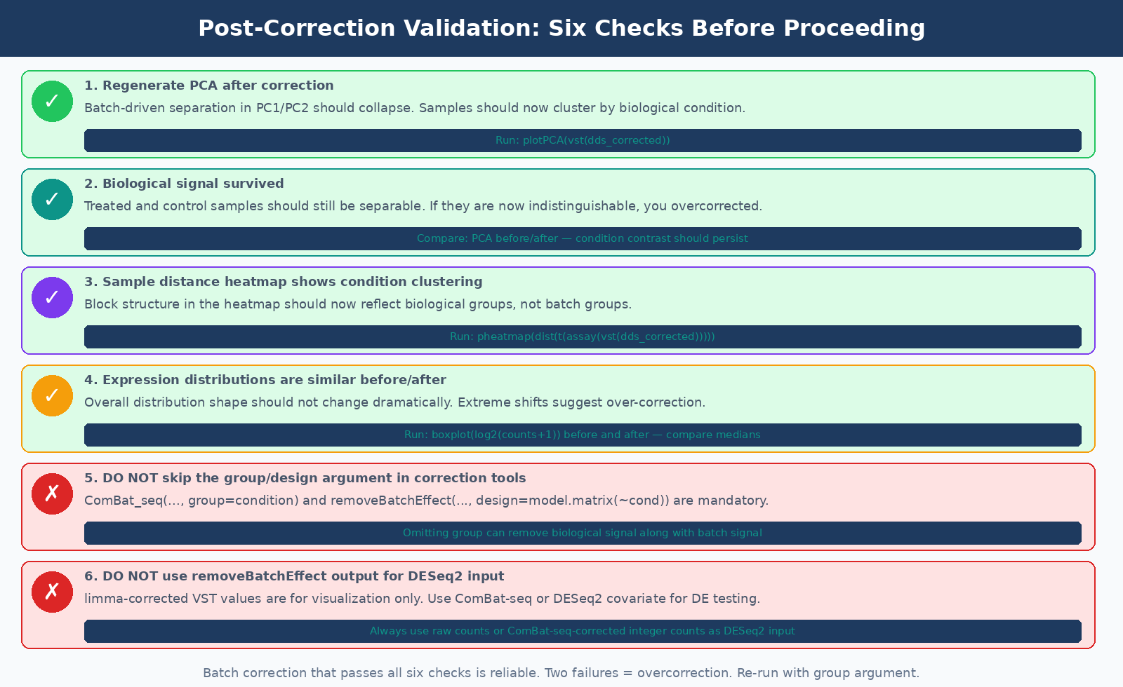
Validating That Correction Worked
Running a correction tool and moving on without validation is a mistake. After applying either ComBat-seq or removeBatchEffect, regenerate your PCA and sample-distance heatmap. The batch structure should have collapsed: samples from the same biological condition should now cluster together, and the batch-driven separation in PC1 or PC2 should be gone or substantially reduced.
Two specific checks worth running:
First, verify that your biological signal survived. If treated and control samples were distinguishable before correction and are now indistinguishable, you may have overcorrected. This is most likely to happen when you forgot to pass the biological group to the correction function.
Second, check that correction did not introduce new artefacts. Plot the distribution of expression values before and after correction. They should look similar in overall shape. If the distributions are dramatically different or contain values that seem biologically implausible, the correction may have been too aggressive.
The goal of batch correction is not to remove all between-sample variation. It is to remove the component of variation attributable to known technical factors, while leaving the component attributable to biological differences intact.
NotchBio handles batch effect detection and modeling automatically. When you upload a multi-batch experiment and include batch information in your sample sheet, the platform runs PCA to confirm batch structure is present, includes batch as a covariate in the DESeq2 design, and flags any confounding between batch and condition before the analysis proceeds. For experiments where batches are fully confounded with condition, NotchBio surfaces this as a design warning so you can make an informed decision before committing to a final analysis. Learn more at notchbio.app.
Further reading
Read another related post
How to Download RNA-Seq Data from GEO and SRA Using sra-tools and pysradb
Step-by-step tutorial for downloading bulk RNA-seq FASTQ files from GEO and SRA. Covers prefetch, fasterq-dump, pysradb metadata extraction, batch downloads, and fixes for common errors.
TutorialHow to Make Volcano Plots and MA Plots in R: ggplot2 and EnhancedVolcano
Step-by-step R tutorial for publication-quality volcano plots and MA plots from DESeq2 results. Covers ggplot2 from scratch, ggrepel gene labeling, EnhancedVolcano, and plot interpretation.
TutorialPCA and Clustering for RNA-Seq QC in Python: Spot Outliers Before DESeq2
Python tutorial: normalize RNA-seq counts, run PCA with scikit-learn, plot interactively with plotly, build a sample distance heatmap, and detect outliers before differential expression.