Experimental Design Mistakes That Kill Your Differential Expression Analysis
The most dangerous problems in RNA-seq are the ones that do not produce errors. Your pipeline runs cleanly, your PCA looks reasonable, and DESeq2 hands you a list of differentially expressed genes. The list looks plausible. You write it up. Six months later, nothing validates. The failures were not in the analysis; they were decisions made before the first sample was extracted.
Experimental design mistakes in RNA-seq tend to be invisible at the computational stage. You cannot detect pseudoreplication by looking at a count matrix. You cannot see a confounded batch effect in a mapping rate. By the time the data reaches your analysis pipeline, the damage is already done. The only remedy is getting the design right before samples go into tubes.
This post covers the five most common experimental design mistakes in bulk RNA-seq and what to do about each of them. If you are debugging a dataset that already exists, pair this with Batch Effects Will Ruin Your RNA-Seq Results and What Is a Count Matrix and Why Does It Matter because design mistakes usually surface there first.
Mistake 1: Treating Sequencing Depth as a Substitute for Replicates
When budgets are tight, the most common tradeoff is: fewer samples, more reads per sample. More depth will make the data better, right? This is wrong, and the evidence for it is unambiguous.
Biological replicates are of greater importance than sequencing depth for differential expression analysis. An increase in the number of replicates tends to return more differentially expressed genes than increasing the sequencing depth. The intuition behind this is sound: DESeq2 and edgeR estimate gene-wise dispersion from the variance across biological replicates. With more replicates, the dispersion estimate is more accurate, and the model is better calibrated. More reads per sample does not help dispersion estimation at all; it only helps with detection of very lowly expressed transcripts.
ENCODE guidelines suggest 30 million single-end reads per sample for a stranded library, but 15 million reads per sample is often sufficient when you have more than three replicates. The dominant contributing factor to reach optimal power is sample size, not sequencing depth, which plateaus for differential expression detection around 20 million reads per sample for most tools (RNA Journal, 2014).
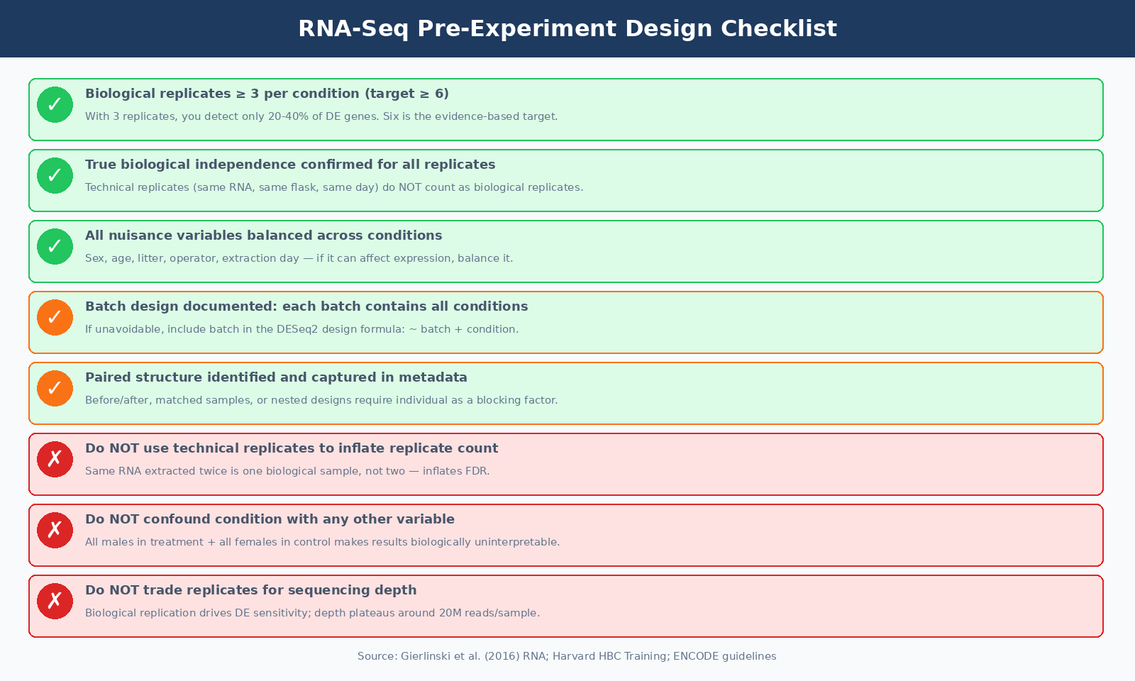
The published evidence on replicate numbers is sobering. With three biological replicates, nine of eleven commonly used DE tools found only 20 to 40 percent of significantly differentially expressed genes identified when using 42 replicates as the ground truth. That recovery rate rises to above 85 percent only for genes changing by more than four-fold. To achieve above 85 percent recovery for all DE genes regardless of fold change requires more than 20 biological replicates. The practical recommendation from that analysis is that at least six biological replicates should be used, rising to at least 12 when capturing low fold-change genes matters (PMC4878611).
In practice, most published studies use three replicates per condition. Three replicates is the minimum that DESeq2 needs to estimate dispersion at all. It is not a number that will give you high sensitivity for modest fold changes. If your budget allows five or six, use them.
Three replicates is a minimum, not a target
With three replicates per condition, you are likely detecting only 20 to 40 percent of all truly differentially expressed genes. That is not a failure of DESeq2; it is a statistical reality about variance estimation at low sample sizes. If your experiment is designed around three replicates and a tight budget, expect modest sensitivity and interpret your gene list accordingly.
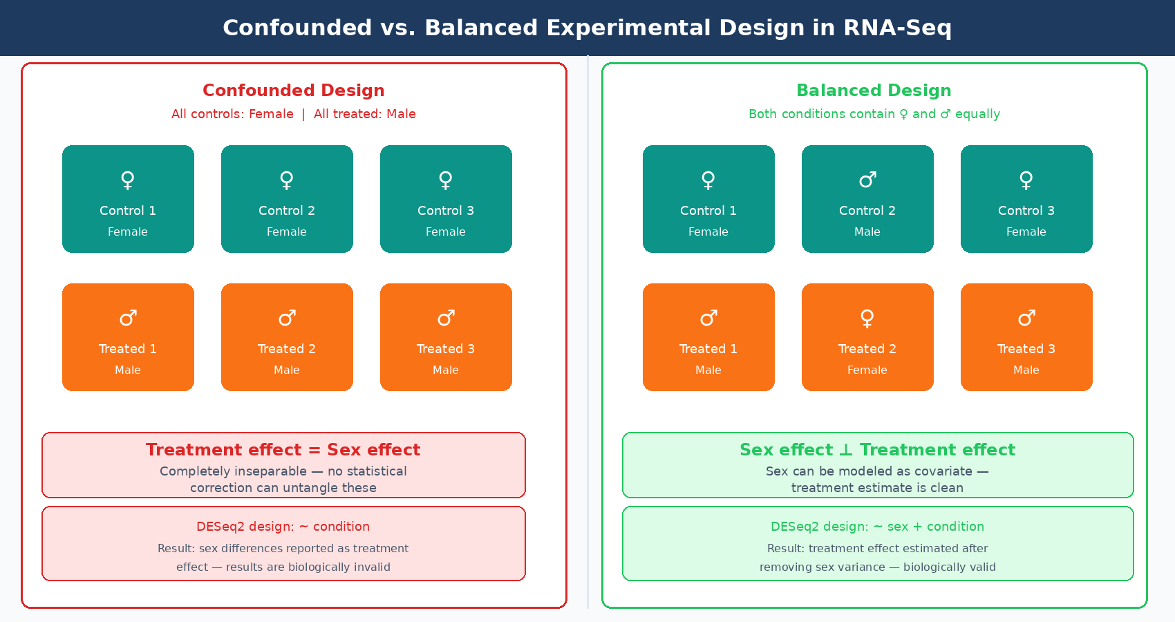
Mistake 2: Confounding Condition with a Nuisance Variable
Confounding is when a variable you did not intend to study becomes inseparable from the variable you did intend to study. In RNA-seq, the classic confounded design is: all control animals are female and all treated animals are male. Now you cannot tell whether your DE genes reflect the treatment or the sex difference, because they are perfectly correlated in your data.
Sex is the most commonly cited example, but the real-world sources of confounding are broader. Age, animal litter, cage, day of sacrifice, RNA extraction batch, library prep operator, and sequencing lane can all become confounders if they are not explicitly balanced across conditions.
A confounded experiment is not recoverable by statistical methods. If all control samples were extracted on day one and all treated samples were extracted on day two, you can try to include batch in your DESeq2 design formula, but you cannot distinguish what is batch from what is treatment. They are completely collinear. The batch term and the treatment term will compete for the same variance, and your estimates will be wrong regardless of how sophisticated your modeling is.
The prevention is simple and must happen at the design stage. For each potential nuisance variable, ask: is this variable balanced across my conditions? If the answer is no for any variable that could plausibly affect gene expression, redesign the experiment.
Mistake 3: Not Accounting for Batch Effects in the Design
Batch effects in RNA-seq are not just common; they are close to universal at scale. Any time samples are processed at different times, by different operators, on different instruments, or across different reagent lots, there is potential for systematic technical variation that has nothing to do with your biological question.
The correct response to batches is not to avoid them; they are often unavoidable in practice. The correct response is to design your experiment so that batches are informative rather than confounded. This means ensuring that each batch contains at least one sample from each experimental condition. If you have four conditions and must run samples across two library prep batches, each batch should include samples from all four conditions.
When batches are balanced across conditions, you can model batch as a covariate in your DESeq2 design formula:
design = ~ batch + conditionThis partitions the batch variance away from the condition estimate, and your DE results reflect biology rather than the technician who ran the library prep. What you cannot recover from is a design where all samples from one condition are in batch one and all samples from another condition are in batch two. That is confounding, not a batch effect, and no statistical model fixes it.
If batches are not known in advance but you suspect their presence, PCA is your detection tool. If your first principal component separates samples by processing date rather than by biological condition, you have a batch effect problem. This is detectable and often correctable after the fact using limma::removeBatchEffect or by including a batch term in the model, but only if the batches are not confounded with condition.
Always include batch in your DESeq2 design formula when batches exist
If samples were processed in separate library prep batches, add batch to your design: ~ batch + condition. This is not optional. Ignoring a known batch variable inflates your false discovery rate, because batch variance leaks into the residual and artificially reduces your dispersion estimates.
Mistake 4: Pseudoreplication
Pseudoreplication is treating non-independent observations as if they were independent replicates. In bulk RNA-seq, the most common form is treating technical replicates as biological replicates. A technical replicate is a second library prepared from the same RNA extraction, or a second extraction from the same tissue sample, or a second sequencing run of the same library. None of these are independent biological replicates. They do not contribute to your estimate of biological variability.
The issue matters more than people realize. When pseudoreplication is used in place of true biological replication, the variance estimate fed into DESeq2 reflects technical variation rather than biological variation. Technical variance is much lower than biological variance, which means the model thinks your data is less variable than it actually is. The result is inflated confidence in your DE calls: p-values are too small, fold changes appear more precise than they are, and your FDR is not what you think it is.
This effect is well-documented in single-cell RNA-seq, where treating each cell as an independent replicate instead of each biological sample can inflate DE gene lists by hundreds of times. The same principle applies in bulk: if your three control wells are from the same flask and the same extraction, they are one biological replicate, not three. A published reanalysis of an Alzheimer’s dataset found that pseudoreplication inflated the number of DEGs by a factor of 549 compared to a properly structured pseudobulk analysis (PMC10695556).
For cell line experiments, which are the most prone to this, a biological replicate must be an independent passage of the cells, processed on a different day, ideally with cells from a different passage number. Sequential wells from the same plate, or duplicate libraries from the same RNA, are not biological replicates.
| What It Is | Is It a Biological Replicate? | Reasoning |
|---|---|---|
| Independent mice from the same strain | Yes | Distinct organisms, distinct biological variation |
| Different cell line passages, different days | Yes | Independent biological events |
| Same RNA, two library preps | No | Technical replicate only |
| Same library, two sequencing runs | No | Technical replicate only |
| Two wells from the same flask, same day | No | Not biologically independent |
| Same sample, different RNA extraction | Borderline | Captures extraction variability but not biological variance |
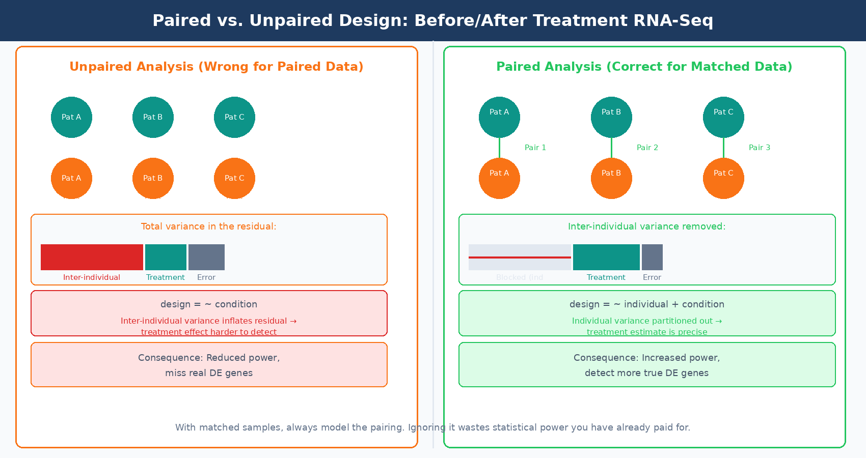
Mistake 5: Ignoring Paired Designs
A paired experimental design is one where samples within a condition are naturally linked: before and after treatment in the same patient, matched tumor and normal tissue from the same individual, or two time points from the same animal. Ignoring this pairing structure in your DESeq2 model is a design mistake that costs you statistical power without causing obvious downstream errors.
In a paired design, much of the between-sample variance in your data reflects differences between individuals rather than the treatment effect. When you do not model the pairing, that individual-level variance goes into the residual and makes the treatment effect harder to detect. When you do model it, you account for the individual as a blocking factor and the treatment estimate becomes more precise.
In DESeq2, a paired design is modeled by including the individual as a factor:
design = ~ individual + conditionWhere individual is a factor variable identifying which samples came from the same person or animal. This removes the between-individual variance from the error term, which can dramatically increase power. The effect size is larger in datasets where inter-individual variation is high relative to the treatment effect, which is common in human tissue studies and clinical samples.
The paired design also affects how you interpret your results. If you run a paired analysis, your fold change estimates reflect the within-individual treatment effect, averaged across individuals. If you run an unpaired analysis on paired data, your fold change estimates are noisier and your p-values are inflated in the wrong direction (too conservative), meaning you will miss real DE genes that a properly specified model would have detected.
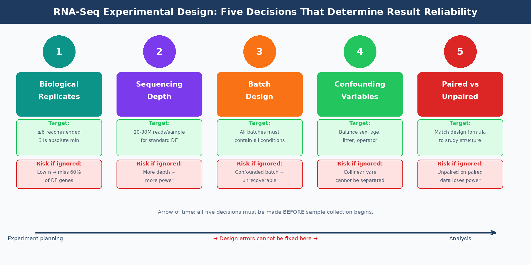
Putting It Together: Design Checklist Before You Start
The six questions you should be able to answer yes to before your first sample is collected:
First, how many biological replicates per condition, and are they true biological replicates with independent derivation and processing? Three is the absolute floor; five or six is the practical target for reasonable sensitivity across fold changes.
Second, are all nuisance variables balanced across conditions? Sex, age, litter, cage, extraction batch, and operator should all be distributed across conditions, not clustered within them.
Third, if batches are unavoidable, is each batch designed to contain at least one sample from each experimental condition? Batch effects you can model are manageable. Batch effects confounded with condition are not.
Fourth, does your experimental question involve a natural pairing between samples? If yes, the design formula must include the blocking factor, and both samples in each pair must be collected and sequenced.
Fifth, do you know your sequencing depth target per sample? For most standard differential expression experiments, 20 to 30 million paired-end reads per sample is the right target. More depth helps only if you are specifically interested in lowly expressed genes or isoform-level analysis.
Sixth, have you pre-registered or documented your analysis plan before seeing the data? This is not strictly a design question, but it is the honest extension of the same principle: decisions made after seeing data are not the same as decisions made before, and mixing the two degrades the integrity of your results.
DESeq2 is a robust tool. It handles low-count genes well, models dispersion accurately across a range of replicate numbers, and its shrinkage estimators help with noisy data. But DESeq2 cannot correct for a confounded design. It cannot add statistical power you decided not to purchase when you cut the replicate count to save money. It cannot distinguish biological variation from batch variation if batches are not modeled. The tool is only as good as the experiment it was handed.
NotchBio runs DESeq2 as part of an automated pipeline from FASTQ to differential expression results. When you upload your samples and specify your experimental design, the platform validates your design matrix, checks for confounding between variables, and flags batch structure before the analysis runs. If your experiment has identifiable design problems, you see them as warnings before you commit to a final analysis run. You can learn more at notchbio.app.
Further reading
Read another related post
What Is a Count Matrix and Why Does It Matter
Raw counts, TPM, FPKM, and DESeq2 normalized values all represent gene expression differently. Here is what each one is, why the differences matter, and which to use for each downstream task.
Research GuideWhy Your Choice of Reference Genome Changes Your Results
GENCODE, Ensembl, UCSC, and RefSeq annotate the same genome differently. Here is how annotation choice affects RNA-seq alignment, quantification, and which genes appear significant.
TutorialTrimming Adapters with Trimmomatic and fastp: A Side-by-Side Walkthrough
When adapter trimming helps, when it hurts, and how to run Trimmomatic and fastp on RNA-seq data with the parameter choices that actually matter.