How to Run DESeq2: A Complete Walkthrough from Count Matrix to Results

DESeq2 has been cited over 60,000 times. It is the closest thing to a standard that bulk RNA-seq differential expression analysis has. That citation count also means there is a lot of outdated tutorial content online, written before the 2018 introduction of apeglm shrinkage or the shift away from betaPrior in the Wald test. This walkthrough reflects current best practice.

This tutorial starts from a count matrix, walks through every step of the DESeq2 pipeline with working R code, explains what each step is actually doing, and ends with a saved, annotated results table ready for downstream pathway analysis. It also covers the design matrix decisions that most tutorials skip.

If you are coming from transcript-level quantification, Importing Salmon Output into R: tximeta, tximport, and DESeq2 Setup is the prerequisite. If you want the conceptual version first, How DESeq2 Actually Works (Without the Math Overload) explains the same model without the code.

What DESeq2 Is Doing Under the Hood

Before running code, it helps to understand the model, because the settings you choose only make sense if you know what problem they are solving.

DESeq2 models raw read counts using a negative binomial distribution: K_ij ~ NB(mu_ij, alpha_i), where K_ij is the count for gene i in sample j, mu_ij is the fitted mean, and alpha_i is a gene-specific dispersion parameter (DESeq2 reference manual). The negative binomial is used instead of a Poisson because RNA-seq count data is overdispersed: the variance exceeds the mean for most genes, particularly at low and moderate expression levels.

The fitted mean mu_ij is composed of a sample-specific size factor s_j and a parameter proportional to the true expression level. The size factor absorbs differences in sequencing depth between samples, so that a gene with 1000 counts in a deeply sequenced sample is not artificially treated as more expressed than the same gene with 500 counts in a shallower sample.

The dispersion parameter alpha_i is what makes DESeq2 powerful for small sample sizes. With three replicates per condition, a gene-specific dispersion estimate from those three values alone is extremely noisy. DESeq2 solves this by borrowing information across all genes: it fits a smooth curve of dispersion versus mean expression across all genes, then shrinks gene-specific estimates toward that curve. Genes with reliable data (high counts, consistent replicates) deviate from the curve; genes with unreliable data are pulled toward it. This step is what allows DESeq2 to produce sensible p-values from three replicates per condition where a simple t-test would completely fail (HBC Training materials).

The final step is a Wald test on the log2 fold change coefficient. DESeq2 divides the estimated LFC by its standard error, producing a z-statistic, and compares it to a standard normal distribution. The resulting p-values are then adjusted for multiple testing using the Benjamini-Hochberg procedure.

How to Load Your Count Matrix into DESeq2

DESeq2 accepts count matrices from several upstream sources. The input must always be raw integer counts, not TPM, FPKM, or any other normalized metric.

If you came from the previous tutorial and have Salmon output imported via tximport, you are already ready:

library(DESeq2)

# From tximport (previous tutorial)
dds <- DESeqDataSetFromTximport(txi, colData = coldata, design = ~ condition)

If you have a raw count matrix from featureCounts, HTSeq-count, or another alignment-based counting tool, use DESeqDataSetFromMatrix:

library(DESeq2)

# Load count matrix (genes x samples, integer values)
count_matrix <- read.csv("results/counts/feature_counts.csv",
                          row.names = 1,
                          check.names = FALSE)

# Verify it looks right
dim(count_matrix)         # e.g., [1] 60000    6
class(count_matrix[1, 1]) # should be integer or numeric
head(count_matrix[, 1:3]) # spot-check a few values

# Sample metadata: must match column names of count_matrix
coldata <- data.frame(
    condition = factor(c("control", "control", "control",
                         "treated", "treated", "treated"),
                       levels = c("control", "treated")),
    row.names = colnames(count_matrix)
)

# Build DESeqDataSet
dds <- DESeqDataSetFromMatrix(
    countData = count_matrix,
    colData   = coldata,
    design    = ~ condition
)

Pre-Filtering: Which Genes to Keep

Before running the model, filter out genes with very low counts. There are two reasons to do this. First, DESeq2 performs independent filtering automatically, but doing a pre-filter reduces memory and speeds up the analysis. Second, genes with zero counts across all samples carry no information and should be removed unconditionally.

# Remove genes with fewer than 10 counts across all samples
# The threshold and the minimum number of samples are both adjustable
keep <- rowSums(counts(dds) >= 10) >= 3
dds  <- dds[keep, ]

# For a study with 3 replicates per group, keeping genes with
# at least 10 counts in at least 3 samples is a sensible default.
# For larger experiments (6+ replicates), you can be more stringent.

cat("Genes before filtering:", nrow(dds) + sum(!keep), "\n")
cat("Genes after filtering:", nrow(dds), "\n")
# Typical: 60,000 → ~18,000 after filtering

Setting the Reference Level in Your Design

DESeq2 uses alphabetical ordering to determine the reference level of a factor by default. For a condition factor with levels control and treated, control comes first alphabetically and is used as the reference automatically. But if your conditions are named differently, set the reference explicitly:

# Confirm or set the reference level
levels(dds$condition)
# [1] "control" "treated"   <- control is already the reference

# If it were wrong, set it explicitly:
# dds$condition <- relevel(dds$condition, ref = "control")

# The reference level is the denominator in the fold change:
# log2(treated / control)
# A positive LFC means higher expression in the treated group

Getting the reference level wrong does not break DESeq2. It just reverses the sign of all your fold changes, which is a common source of confusion when interpreting results.

How to Run DESeq2 Step by Step

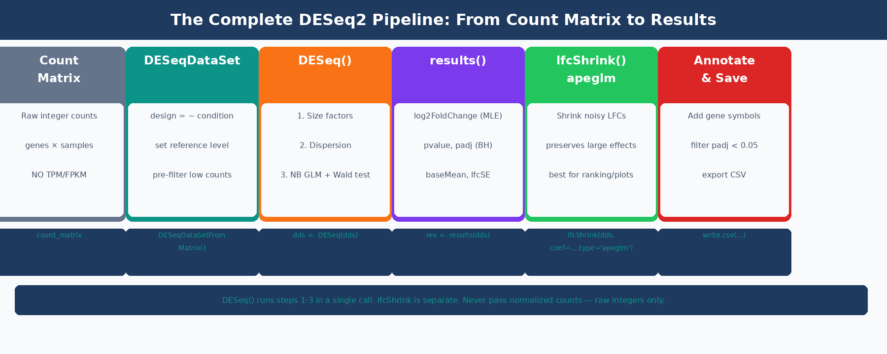
The DESeq() function wraps the full pipeline into a single call:

# Run DESeq2
# Prints: estimating size factors, estimating dispersions,
#         fitting model and testing
dds <- DESeq(dds)

That single line executes three sequential steps. You should understand what each one does.

Step 1: Size Factor Estimation

# Inspect the size factors after DESeq() runs
sizeFactors(dds)
#   ctrl_1  ctrl_2  ctrl_3 treat_1 treat_2 treat_3
#   1.032   0.978   1.041   0.962   1.084   0.891

# Size factors near 1.0 indicate balanced library sizes.
# A sample with a size factor of 0.5 had roughly half as many
# counts as the geometric mean, so its counts are divided by 0.5
# (doubled) during normalization.

DESeq2 calculates size factors using the median-of-ratios method: for each sample, it computes the ratio of each gene’s count to the geometric mean of that gene’s counts across all samples, then takes the median of those ratios. This is robust to outlier genes and works well when only a minority of genes are differentially expressed.

Step 2: Dispersion Estimation

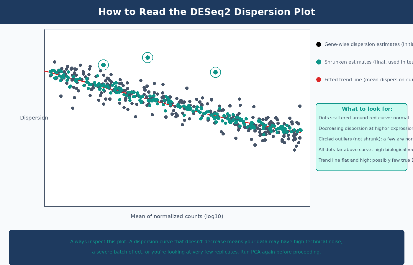
The dispersion plot is the most informative diagnostic in the DESeq2 pipeline. Always inspect it:

# Visualize dispersion estimates
plotDispEsts(dds)

In a clean dataset you expect to see: gene-wise dispersion estimates (black dots) scattered around a fitted trend line (red curve), with final shrunken estimates (blue dots) pulled toward the curve. The spread around the curve decreases at higher expression levels. A plot where most points are far above the trend line, or where the trend line is flat and high, indicates a dataset with high biological variability or too few replicates.

Step 3: Wald Test and p-Value Calculation

After fitting the negative binomial model, DESeq2 performs a Wald test on each gene’s LFC coefficient. The test asks: is the estimated LFC significantly different from zero, given the model’s estimate of its uncertainty?

The Wald test statistic is the LFC divided by its standard error. Large positive or negative values indicate genes where the fold change is precisely estimated and large relative to its uncertainty. The resulting p-values are then adjusted for multiple testing using Benjamini-Hochberg false discovery rate correction.

How to Extract and Read DESeq2 Results

# Extract results table
res <- results(dds)

# Summary of significant results at the default alpha threshold
summary(res)
# out of 18,234 with nonzero total read count
# adjusted p-value < 0.1:
# LFC > 0 (up)       : 412, 2.3%
# LFC < 0 (down)     : 388, 2.1%
# outliers [1]       :  12, 0.1%
# low counts [2]     : 943, 5.2%
# (mean count < 5)

# Look at the first few rows
head(res[order(res$padj), ])

The results table has six columns. Understanding all of them prevents common misinterpretations:

Specifying Contrasts for Multi-Condition Experiments

When your experiment has more than two groups, use the contrast argument to specify which comparison you want:

# Three-condition experiment: control, dose_low, dose_high
# After running DESeq(dds)...

# All available contrasts
resultsNames(dds)
# [1] "Intercept"
# [2] "condition_dose_low_vs_control"
# [3] "condition_dose_high_vs_control"

# Extract specific contrasts
res_low_vs_ctrl  <- results(dds,
    contrast = c("condition", "dose_low",  "control"),
    alpha    = 0.05)   # sets the threshold for plotMA and summary()

res_high_vs_ctrl <- results(dds,
    contrast = c("condition", "dose_high", "control"),
    alpha    = 0.05)

# Comparison not in resultsNames (e.g., high vs low)
# requires relevel or using the list syntax
res_high_vs_low  <- results(dds,
    contrast = c("condition", "dose_high", "dose_low"),
    alpha    = 0.05)

Why You Should Always Apply LFC Shrinkage with apeglm

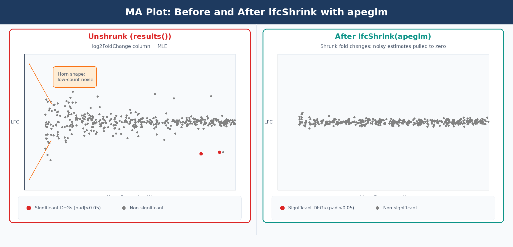
The log2FoldChange column in the raw results() output is a maximum likelihood estimate. For genes with low counts or high dispersion, this estimate is very noisy: a gene with 2 counts in control and 8 counts in treated has an apparent log2FC of 2.0, but the uncertainty on that estimate is enormous. When you rank genes by absolute fold change for a volcano plot or GSEA input, these noisy estimates from lowly expressed genes dominate the top of the list.

lfcShrink with the apeglm method solves this problem. It applies a Cauchy prior to the LFC estimates, pulling unreliable estimates toward zero without shrinking genuine large fold changes. The apeglm method improves on the previous normal-prior shrinkage estimator by using a heavy-tailed prior that preserves large, reliable fold changes while aggressively shrinking noisy small-count estimates (Zhu, Ibrahim, and Love, 2018, Bioinformatics).

library(apeglm)

# Check available coefficient names
resultsNames(dds)
# [1] "Intercept"  "condition_treated_vs_control"

# Apply apeglm shrinkage
res_shrunk <- lfcShrink(
    dds,
    coef = "condition_treated_vs_control",
    type = "apeglm"
)

# Compare raw vs shrunk fold changes for a low-count gene
gene_example <- "ENSG00000000003"
cat(sprintf("Raw LFC:    %.3f (SE: %.3f)\n",
    res[gene_example, "log2FoldChange"],
    res[gene_example, "lfcSE"]))
cat(sprintf("Shrunk LFC: %.3f\n",
    res_shrunk[gene_example, "log2FoldChange"]))
# Low-count genes: raw LFC of ±3 shrinks to ±0.2
# High-count genes: shrunk LFC is nearly identical to raw

Once you have the shrunk table, How to Make Volcano Plots and MA Plots in R: ggplot2 and EnhancedVolcano and What Is GSEA and Why Does It Beat a Simple DEG List cover the two most common downstream interpretation steps.

How to Filter DESeq2 Results by Adjusted p-value and Fold Change

After obtaining shrunk results, apply your significance thresholds and save:

# Convert to data frame for easier manipulation
res_df <- as.data.frame(res_shrunk)

# Add gene name column (if using Ensembl IDs, add symbol mapping)
res_df$gene_id <- rownames(res_df)

# Filter: significant at padj < 0.05 AND |LFC| > 1 (2-fold change)
sig_genes <- subset(res_df,
    padj < 0.05 & abs(log2FoldChange) > 1)

cat(sprintf("Total genes tested: %d\n", nrow(res_df)))
cat(sprintf("Significant DEGs (padj<0.05, |LFC|>1): %d\n", nrow(sig_genes)))
cat(sprintf("  Up:   %d\n", sum(sig_genes$log2FoldChange > 0)))
cat(sprintf("  Down: %d\n", sum(sig_genes$log2FoldChange < 0)))

# Sort by adjusted p-value
sig_genes <- sig_genes[order(sig_genes$padj), ]

# Save full results (including non-significant genes)
# Include these for GSEA, which needs a ranked list of all genes
write.csv(res_df, "results/deseq2_all_genes.csv", row.names = FALSE)

# Save significant DEGs only
write.csv(sig_genes, "results/deseq2_significant_degs.csv", row.names = FALSE)

The |LFC| > 1 threshold is a fold change of 2 in either direction. Whether this is appropriate depends on your experiment. For cell line perturbations with strong expected effects, this is a reasonable starting threshold. For subtle treatments or clinical samples where modest changes are biologically meaningful, you might use |LFC| > 0.5 or no LFC filter at all, relying solely on padj.

Adding Gene Symbols to Your Results Table

Ensembl gene IDs are not readable in final reports. Map them to gene symbols using AnnotationDbi:

library(AnnotationDbi)
library(org.Hs.eg.db)   # Human; use org.Mm.eg.db for mouse

# Map ENSEMBL IDs to gene symbols
# Remove version suffixes first (ENSG00000000003.14 -> ENSG00000000003)
gene_ids_clean <- gsub("\\..*", "", res_df$gene_id)

res_df$symbol <- mapIds(
    org.Hs.eg.db,
    keys     = gene_ids_clean,
    column   = "SYMBOL",
    keytype  = "ENSEMBL",
    multiVals = "first"   # for genes with multiple symbols, take first
)

# Check mapping rate
cat(sprintf("Genes with symbol mapping: %d / %d (%.0f%%)\n",
    sum(!is.na(res_df$symbol)),
    nrow(res_df),
    100 * mean(!is.na(res_df$symbol))))
# Expect 85-95% mapping rate with GENCODE annotations

# Final table with readable columns
results_final <- res_df[, c("gene_id", "symbol", "baseMean",
                              "log2FoldChange", "lfcSE",
                              "pvalue", "padj")]
results_final <- results_final[order(results_final$padj), ]

write.csv(results_final,
          "results/deseq2_results_annotated.csv",
          row.names = FALSE)

Running a Full DESeq2 Pipeline: Putting It Together

Here is the complete pipeline in a single script:

#!/usr/bin/env Rscript
# Input: count matrix CSV + sample metadata CSV
# Output: annotated results CSV

library(DESeq2)
library(apeglm)
library(AnnotationDbi)
library(org.Hs.eg.db)

# ── 1. Load data ─────────────────────────────────────────────
count_matrix <- read.csv("results/counts/counts.csv",
                          row.names = 1, check.names = FALSE)

coldata <- read.csv("data/sample_metadata.csv",
                    row.names = 1, stringsAsFactors = TRUE)

# Ensure sample order matches
stopifnot(all(colnames(count_matrix) == rownames(coldata)))

# ── 2. Build DESeqDataSet ────────────────────────────────────
dds <- DESeqDataSetFromMatrix(
    countData = count_matrix,
    colData   = coldata,
    design    = ~ condition
)

# Set reference level (control is reference)
dds$condition <- relevel(dds$condition, ref = "control")

# Pre-filter: keep genes with >= 10 counts in >= 3 samples
keep <- rowSums(counts(dds) >= 10) >= 3
dds  <- dds[keep, ]
message(sprintf("After filtering: %d genes", nrow(dds)))

# ── 3. Run DESeq2 ────────────────────────────────────────────
dds <- DESeq(dds)

# Diagnostic: inspect dispersion plot
pdf("results/deseq2_dispersion_plot.pdf")
plotDispEsts(dds)
dev.off()

# ── 4. Extract results ───────────────────────────────────────
coef_name <- resultsNames(dds)[2]   # first non-intercept coefficient
message(sprintf("Extracting results for: %s", coef_name))

# Unshrunk results (for significance testing)
res_raw    <- results(dds, alpha = 0.05)

# Shrunk results (for LFC estimates, visualization, ranking)
res_shrunk <- lfcShrink(dds, coef = coef_name, type = "apeglm")

# ── 5. Annotate and save ─────────────────────────────────────
res_df        <- as.data.frame(res_shrunk)
res_df$gene_id <- rownames(res_df)

# Strip version from Ensembl IDs
gene_ids_clean <- gsub("\\..*", "", res_df$gene_id)
res_df$symbol  <- mapIds(org.Hs.eg.db,
                          keys      = gene_ids_clean,
                          column    = "SYMBOL",
                          keytype   = "ENSEMBL",
                          multiVals = "first")

res_df <- res_df[order(res_df$padj, na.last = TRUE), ]

# Save: full ranked list for GSEA
write.csv(res_df,
          "results/deseq2_all_genes_ranked.csv",
          row.names = FALSE)

# Save: significant DEGs only
sig <- subset(res_df, padj < 0.05 & abs(log2FoldChange) > 1)
write.csv(sig,
          "results/deseq2_significant_degs.csv",
          row.names = FALSE)

message(sprintf("Done. %d DEGs (padj<0.05, |LFC|>1).", nrow(sig)))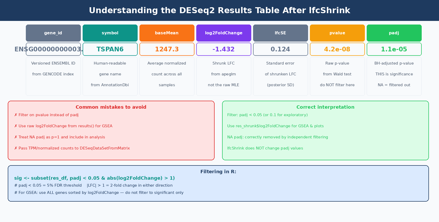

Common DESeq2 Errors and How to Fix Them

estimateSizeFactors error: every gene contains at least one zero: this usually means your count matrix has samples or genes with all zeros, or you are passing a non-integer matrix. Check any(is.na(counts(dds))) and class(counts(dds)[1,1]).

coef argument not in resultsNames(dds): you passed a string to lfcShrink that does not match any coefficient name. Run resultsNames(dds) first and copy the exact string.

replacement has length zero in relevel: your factor has only one level, meaning all samples are in the same condition. Check levels(dds$condition).

All padj values are NA: your filter threshold is too aggressive, leaving no genes with sufficient counts for testing. Relax the filtering step or check whether your count matrix loaded correctly.

NotchBio runs the full DESeq2 pipeline internally, from tximeta import through apeglm shrinkage and gene symbol annotation, returning a ranked results table alongside your QC report. If you want to run the analysis without managing the R environment and package versions, start at notchbio.app.