STAR vs HISAT2 vs Salmon: Which Aligner Should You Use?
The aligner choice is one of the first real decisions in a bulk RNA-seq pipeline, and it is also one of the most misunderstood. Researchers either default to whatever their institution used before them, or they read one benchmark paper and commit to a single tool without understanding why the comparison came out the way it did.
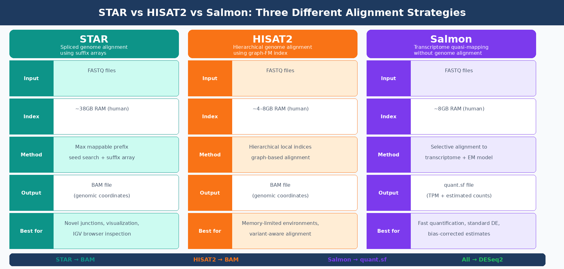
The three tools that dominate modern bulk RNA-seq are STAR, HISAT2, and Salmon. STAR and HISAT2 are genome aligners: they map reads to a reference genome and produce BAM files. Salmon is not an aligner in the same sense at all. It maps reads to a transcriptome and skips genome alignment entirely. These are fundamentally different operations, and that difference matters for what each tool can and cannot do.
This post explains how each tool works, what it produces, where each one has a genuine advantage, and which combination is right for which experiment. If you want the upstream context for why annotation choice changes these results, pair this with Why Your Choice of Reference Genome Changes Your Results. If you already know Salmon is the route you want, How to Quantify RNA-Seq Reads with Salmon is the practical follow-up.
What Alignment Actually Does
Before comparing tools, it is worth being precise about what alignment means in the RNA-seq context.
When you align RNA-seq reads to a genome, you are determining the genomic coordinates where each read originated. This is non-trivial for RNA-seq specifically, because your reads were sequenced from mature messenger RNA — which means the sequences crossed exon-exon junctions that do not exist in genomic DNA. A 100bp read spanning a splice junction might have 80bp from one exon and 20bp from the next, with an intron of thousands of bases between them in the genome. A splice-aware aligner has to recognize this, split the read, and map each part to the correct exon.
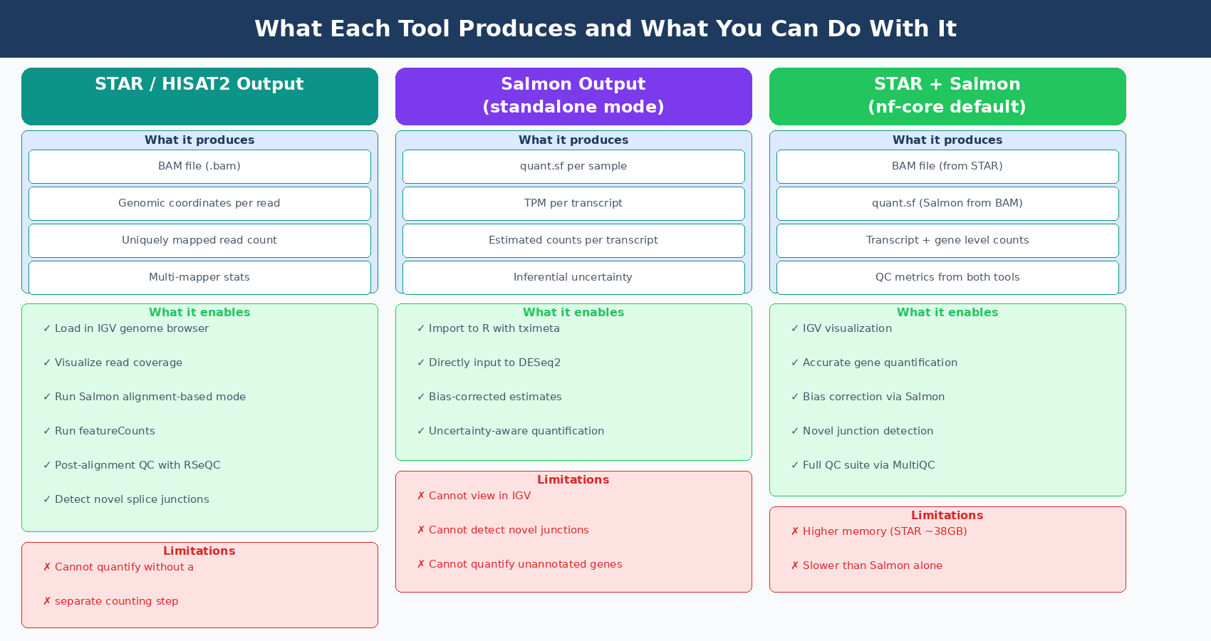
Genome alignment gives you positional information. You can load a BAM file into IGV and look at reads piling up on your gene of interest. You can see the coverage pattern, identify where reads drop off, spot an exon that is missing in your knockout. This is scientifically valuable and has no substitute.
Transcriptome mapping, the approach Salmon uses, asks a different question. Instead of “where on the genome does this read map?”, it asks “which transcripts are compatible with this read?” You are not computing genomic coordinates. You are computing a probability distribution over all transcripts in your reference that could have generated each read, and then using that distribution to estimate transcript abundances. This is faster and uses less memory, but you lose the positional information entirely. You cannot load a Salmon output into IGV.
Neither approach is universally better. They answer different questions with different tradeoffs.
STAR: The High-Accuracy Genome Aligner
STAR (Spliced Transcripts Alignment to a Reference) is the current standard for splice-aware genome alignment in bulk RNA-seq. It has been cited as the default aligner in the nf-core/rnaseq pipeline and has been shown to have high accuracy, outperforming other genome aligners by more than a factor of 50 in mapping speed compared to older tools like TopHat (nf-core documentation). Kallisto and Salmon and STAR provided superior mapping performance, were quickest, and had the smallest output file size compared to other tested aligners (FAA benchmarking study).
STAR’s core algorithm uses a maximal mappable prefix search through suffix arrays to find where each read maps. Its seed-searching step locates a maximal mappable prefix beginning with the first base of a read, then the algorithm identifies splice junction locations within each read sequence. A key advantage is that STAR can detect splice junctions without a junction database, discovering novel junctions purely from the read data itself.
The output of a STAR run is a BAM file: a compressed binary file containing the genomic coordinates of every aligned read. You then feed this BAM file to a counting tool like featureCounts or use Salmon in alignment-based mode to quantify transcript abundances from the BAM file itself. The nf-core/rnaseq pipeline’s default route is STAR alignment followed by Salmon quantification, combining STAR’s precise alignment with Salmon’s statistical quantification model.
The cost is memory. STAR requires a lot of memory to run, typically around 38GB for the human GRCh37 reference genome (nf-core/rnaseq documentation). This number is not negotiable: STAR loads its genome index entirely into RAM before alignment begins. On a shared HPC cluster this is rarely a problem, but on a desktop workstation or a small cloud instance, 38GB of RAM is a hard requirement.
HISAT2: Lighter Memory, Good for Resource-Constrained Environments
HISAT2 (Hierarchical Indexing for Spliced Alignment of Transcripts 2) uses a fundamentally different indexing strategy than STAR. Rather than a single global suffix array, HISAT2 builds a hierarchical index using graph Ferragina-Manzini indexing, which organizes the genome into many small local indices rather than one large global one. This allows HISAT2 to represent and search genomic variants, haplotypes, and SNPs within the index itself — a capability that made it particularly attractive for variant-aware alignment.
The practical result is a much smaller memory footprint. The HISAT2 index for the human genome requires roughly 4 to 8GB of RAM rather than STAR’s 38GB. This makes HISAT2 the right choice when you are operating on memory-limited hardware, such as standard desktop machines, smaller cloud instances, or HPC queue slots with memory limits.
HISAT2 is also generally faster than STAR in wall time per sample. HISAT2 is far faster than STAR in running human paired-end samples on standard hardware because HISAT2 is not resource demanding (benchmarking study). STAR can compensate with superior multi-threading on high-core-count servers, but HISAT2’s speed advantage is consistent on standard hardware configurations.
The tradeoff is accuracy in some edge cases. STAR uses maximum mappable seed search combined with suffix arrays, allowing it to rapidly achieve high mapping efficiency, while HISAT2 employs hierarchical indexing that results in slightly lower mapping efficiency (benchmarking, ResearchGate 2023). One specific concern is retrogene loci: a comparison of STAR and HISAT2 on clinical breast cancer data found that HISAT2 was prone to misalign reads to retrogene genomic loci, while STAR generated more precise alignments (PMC6617288). For most standard experiments this is not a meaningful issue, but for studies where retrogenes or pseudogenes are biologically relevant, it is worth noting.
HISAT2 is the nf-core fallback for memory-constrained environments
The nf-core/rnaseq pipeline documentation states: use the HISAT2 aligner if your compute environment does not have sufficient memory to run STAR. This is a practical recommendation, not a performance endorsement. Both tools produce valid results for standard differential expression analysis. STAR is the default because it is more accurate in edge cases and integrates more cleanly with Salmon quantification.
Salmon: Skip the Genome Entirely
Salmon does not align reads to a genome. It uses a technique the developers call selective alignment (or, in older versions, quasi-mapping): reads are matched against a transcriptome index using an FMD-indexed suffix array to find compatible transcripts, and then a statistical model estimates transcript abundances from those compatibility assignments.
The model Salmon uses is more sophisticated than a simple count. It estimates a probability distribution over transcripts that accounts for the read’s sequence content, its position within a transcript, and its orientation. Salmon also models and corrects for biases including GC content bias, fragment length bias, and positional effects — sources of systematic error that affect alignment-based quantification but that most counting tools do not correct for.
Speed and memory are dramatically lower. A paired-end library with 22 million reads runs in 3.5 minutes on a single CPU core using 8GB of memory (NYU Genomics Core). Kallisto (which uses the same basic approach) was shown to be 2.6 times faster than STAR in single-cell workflows, using in some cases 15 times less RAM (Biostars, Lior Pachter). For bulk RNA-seq, the speed and memory differences are similarly dramatic.
Salmon outputs a quant.sf file per sample containing transcript-level abundance estimates in TPM and estimated counts. These are not genome-level BAM files. There are no genomic coordinates. You cannot visualize Salmon output in a genome browser. What you get instead is a probabilistically estimated expression table that you import into R using tximeta or tximport and then feed directly to DESeq2.
The fundamental limitation is that Salmon only quantifies what is in its transcriptome index. It cannot detect novel splice junctions. It cannot quantify transcripts that are not in the reference annotation. If your biological question involves a knockout that creates a novel fusion transcript, or a variant that disrupts a canonical splice site and creates a new isoform, Salmon will not detect it. STAR would, because it can discover novel junctions from the read data itself.
Salmon cannot quantify transcripts outside its reference annotation
Salmon and Kallisto only map to the transcriptome rather than the genome, and their results are only as good as the transcript annotation provided as input. They cannot be used for finding new genes, transcripts, or splice forms. If your experiment involves engineered cell lines with novel constructs, virally transduced sequences, or you expect biologically significant novel isoforms, use STAR.
How the Results Compare
When all three approaches are used on the same data, how different are the expression estimates?
The answer is: for most genes, very similar. A study comparing seven different mappers including STAR, HISAT2, Salmon, and kallisto found correlation coefficients between 0.977 and 0.997 across raw count tables from all methods, with kallisto and Salmon showing the highest similarity at 0.9999 (PMC7084517). For typical differential expression analysis of well-expressed genes, the choice of tool matters less than most researchers assume.
The differences concentrate in lowly expressed genes. STAR and HISAT2 showed higher variance relative to other mappers specifically for lowly expressed genes. Salmon’s probabilistic model, which explicitly handles multi-mapping uncertainty, tends to distribute reads more fairly among competing transcripts. This makes Salmon preferable for studies where quantifying lowly expressed transcripts accurately matters.
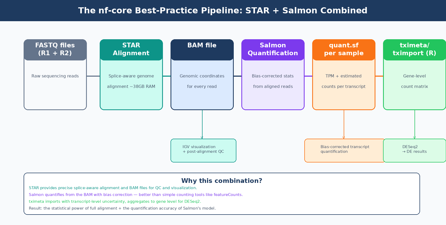
For DE analysis outcomes: the general recommendation from authors of benchmarking studies is to prefer tools that use statistical modules, like Salmon and RSEM, over simple counting tools like featureCounts, considering them more reliable (NAR Genomics and Bioinformatics, 2024). The current nf-core best practice — STAR alignment combined with Salmon quantification — gets the best of both: precise genomic alignment from STAR with Salmon’s statistical quantification applied to the aligned reads.
| Feature | STAR | HISAT2 | Salmon (standalone) |
|---|---|---|---|
| Alignment type | Genome (splice-aware) | Genome (splice-aware) | Transcriptome (quasi/selective) |
| Output | BAM file | BAM file | quant.sf (TPM + counts) |
| RAM requirement (human) | ~38GB | ~4–8GB | ~8GB |
| Speed | Fast (benefits from many threads) | Fast (less thread-hungry) | Extremely fast |
| Novel splice junctions | Detects | Detects (less accurately) | Cannot detect |
| IGV visualization | Yes | Yes | No |
| Bias correction | Limited (via Salmon mode) | Limited | Built-in (GC, fragment length) |
| Multi-mapping handling | Discards by default | Discards by default | Probabilistic redistribution |
| DE analysis input | Requires counting step | Requires counting step | tximport → DESeq2 directly |
| Recommended for | Standard DE, novel junctions | Memory-limited environments | Fast turnaround, well-annotated organisms |
The nf-core Recommendation and Why It Makes Sense
The nf-core/rnaseq pipeline, which has become the de facto standard for reproducible bulk RNA-seq analysis, uses STAR as its default aligner and Salmon as its default quantification tool. The default route, --aligner star_salmon, runs STAR to produce genome-level BAM files, then runs Salmon on those BAM files to produce transcript-level abundance estimates. The BAM files are retained for QC metrics and visualization. The Salmon quant.sf files are imported by tximport for DESeq2.
This combination is well-motivated. STAR provides accurate splice-aware alignment and the BAM files needed for genome browser inspection and post-alignment QC. Salmon then applies its bias-corrected statistical model to quantify from those alignments rather than using a simple counting tool like featureCounts. You get both the precise positional information of full alignment and the statistical sophistication of Salmon’s quantification model.
The alternative in nf-core is to run Salmon as a pure pseudoaligner (--pseudo_aligner salmon), bypassing genome alignment entirely. This is approximately ten times faster and uses substantially less memory, and for a well-annotated human or mouse experiment where novel isoform discovery is not a goal, it produces results that are functionally equivalent for DE analysis. If you take that route, the next step is usually importing Salmon output into R with tximeta or tximport.
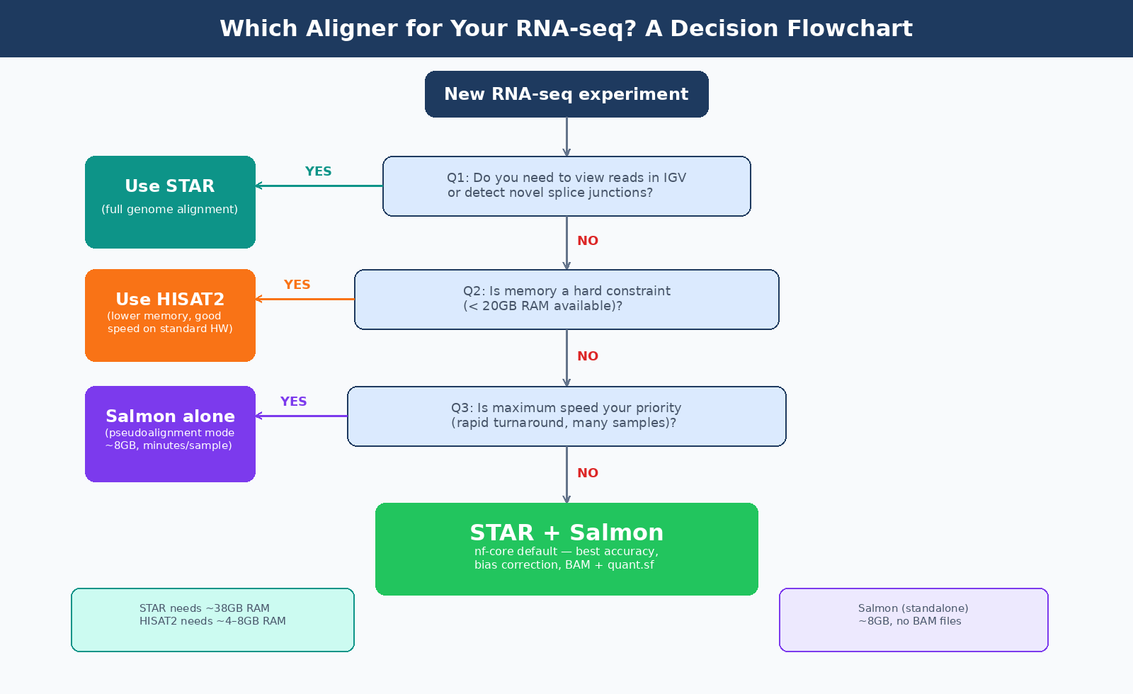
Which route to choose depends on your experimental context. Three questions determine it:
Do you need to visualize reads in a genome browser? If yes, use STAR. You need BAM files for IGV.
Do you need to detect novel splice junctions or quantify transcripts not in the reference annotation? If yes, use STAR. Salmon cannot help here.
Is memory or speed a constraint? If your compute environment cannot provide 38GB of RAM, use HISAT2 for alignment or use Salmon as a pure pseudoaligner.
For everything else — the majority of standard bulk RNA-seq differential expression experiments — the STAR + Salmon combination or Salmon alone will give you reliable results.
A Note on Quantification Tools
Choosing an aligner is only half the decision when using STAR or HISAT2. You also need a counting tool to convert BAM files into gene-level counts. The main options are featureCounts, HTSeq-count, and Salmon in alignment-based mode.
The general recommendation in current best-practice workflows is to avoid featureCounts for de novo quantification and instead use Salmon’s alignment-based mode, because Salmon applies its statistical model even when given pre-aligned BAM files. The nf-core pipeline dropped featureCounts in version 3.x pipelines precisely because featureCounts presents disadvantages for organisms where gene splicing occurs (NAR Genomics and Bioinformatics, 2024).
In practice: if you run STAR, use Salmon in alignment-based mode (salmon quant --alignments) rather than featureCounts. You get Salmon’s bias correction and probabilistic multi-mapping handling applied to your genome-aligned reads. This is what the nf-core pipeline implements, and it produces consistently better quantification accuracy than simple overlap counting.
The Bottom Line
For a standard bulk RNA-seq experiment with human or mouse data, sufficient compute resources (at least 40GB RAM available), and a goal of differential expression analysis: use STAR for alignment and Salmon for quantification, either directly through the nf-core/rnaseq pipeline or by running the two steps separately.
If memory is genuinely constrained: HISAT2 is a well-validated fallback that uses a fraction of STAR’s RAM and produces results that are comparable for most experimental contexts.
If you need maximum speed for a routine DE experiment against a well-annotated organism and do not need BAM files: Salmon alone in pseudoalignment mode runs in minutes and produces expression estimates equivalent to the STAR route for most purposes.
The choice matters less than most researchers think for the final DE gene list. It matters a great deal for what secondary analyses you can run: novel junction discovery, isoform-level analysis, and genome browser visualization all require a BAM file, and only STAR and HISAT2 produce one.
NotchBio runs the STAR plus Salmon pipeline by default, with HISAT2 available as an alternative for experiments where memory constraints require it. The same tximeta-based import and DESeq2 analysis runs downstream regardless of which aligner is used. If you want to run a complete, reproducible alignment-to-results pipeline without configuring each tool, start at notchbio.app.
Further reading
Read another related post
How to Run FastQC and MultiQC on Raw RNA-Seq Reads
A hands-on guide to automating RNA-seq QC across dozens of samples using FastQC and MultiQC, with bash and Python scripts for parsing and flagging failures.
Research GuideRaw Reads to Counts: The Bulk RNA-Seq Pipeline Explained
A practical breakdown of every computational step in bulk RNA-seq: from FASTQ quality control through trimming, alignment, and quantification to your final count matrix.
Research GuideBatch Effects Will Ruin Your RNA-Seq Results
Batch effects silently corrupt bulk RNA-seq data. Learn how to detect them, why they happen, and which correction methods actually work.