How to Quantify RNA-Seq Reads with Salmon: Index, Quant, and Import to R

Most bulk RNA-seq pipelines still reach for alignment by default: STAR generates a BAM file, featureCounts tallies reads over exons, and the resulting matrix goes into DESeq2. That workflow is perfectly valid, but it takes tens of gigabytes of RAM, hours of wall time per run, and produces intermediate files you probably never open again. For the majority of standard differential expression studies, Salmon quantifies more accurately in a fraction of the time.

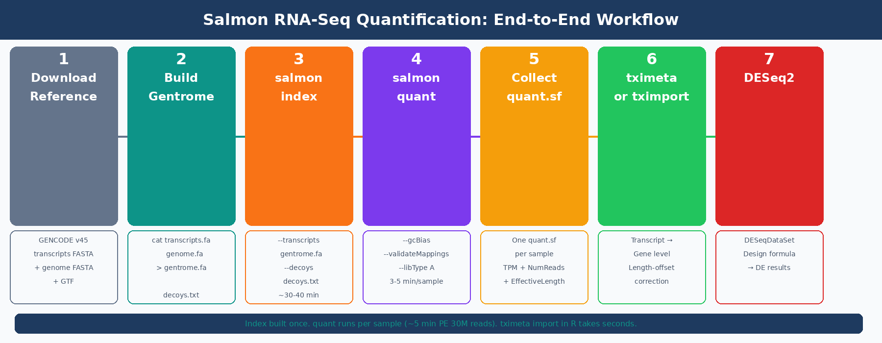
This tutorial walks through the complete Salmon workflow: building a decoy-aware transcriptome index, running quantification on paired-end FASTQ files, understanding what the output files contain, and importing everything into R for DESeq2. By the end, you will have a working pipeline you can drop into any project.

If you are still deciding whether Salmon is the right upstream tool, compare it with STAR vs HISAT2 vs Salmon: Which Aligner Should You Use? and keep Why Your Choice of Reference Genome Changes Your Results in mind when building the index. Once the quant.sf files exist, Importing Salmon Output into R: tximeta, tximport, and DESeq2 Setup is the next handoff.

How Salmon Quantification Works (and Why It Is Faster Than Alignment)

Before running commands, it helps to understand what Salmon is actually doing, because it differs substantially from a genome aligner.

Traditional aligners like STAR find the exact genomic coordinates where each read maps. This requires a genome-scale index, a base-by-base dynamic programming alignment for each read, and a BAM file to store all the results. For a human sample, the index alone consumes about 38GB of RAM.

Salmon uses selective alignment: instead of computing precise genomic coordinates, it determines which transcripts in the reference are compatible with each read, then uses a statistical model to estimate abundances. The model accounts for GC content bias, positional bias, and fragment length distribution, all sources of systematic error that naive counting misses (Salmon documentation, COMBINE-lab). This produces transcript-level TPM values and estimated counts simultaneously, in minutes rather than hours.

The key constraint: Salmon only sees what is in its transcriptome index. It cannot detect novel splice junctions or transcripts missing from the annotation. For standard differential expression against a well-annotated organism, that is not a limitation. For experiments where novel isoform discovery is the goal, use STAR.

How to Install Salmon

Conda is the cleanest installation method. It handles all dependencies and keeps Salmon isolated from your system Python.

# Create a dedicated environment
conda create -n salmon -c conda-forge -c bioconda salmon -y

# Activate
conda activate salmon

# Verify
salmon --version
# salmon 1.10.0

If you are on an HPC cluster, check for a module first:

module spider salmon
module load salmon/1.10.0

The Salmon GitHub releases page also provides pre-compiled binaries if conda is not available in your environment.

How to Build a Salmon Index (Decoy-Aware Method)

The index is built once per reference transcriptome version and reused across all samples. There are two ways to build it: a cDNA-only index (fast, small, slightly less accurate) and a decoy-aware index using the full genome (slower to build, more accurate, recommended for production use).

Why use a decoy-aware index? Reads from genomic regions that share sequence similarity with annotated transcripts can be spuriously mapped to those transcripts if the genome is not in the index. Including the genome as a decoy tells Salmon: if a read maps better to a genomic region than to any transcript, discard it rather than counting it. Accounting for fragments of unexpected origin can improve transcript quantification, particularly for gene families and pseudogenes (Salmon GitHub).

The nf-core/rnaseq pipeline uses the full genome as the decoy by default when running Salmon in pseudoalignment mode (nf-core docs).

Step 1: Download the Reference Files

For human GRCh38, use GENCODE for both the transcript FASTA and the genome FASTA, so chromosome naming is consistent (both use the chr prefix).

mkdir -p references && cd references

# Transcript FASTA (cDNA sequences)
wget https://ftp.ebi.ac.uk/pub/databases/gencode/Gencode_human/release_45/\
gencode.v45.transcripts.fa.gz

# Genome FASTA (primary assembly only, not patches or alt contigs)
wget https://ftp.ebi.ac.uk/pub/databases/gencode/Gencode_human/release_45/\
GRCh38.primary_assembly.genome.fa.gz

# GTF annotation (needed later for tx2gene mapping)
wget https://ftp.ebi.ac.uk/pub/databases/gencode/Gencode_human/release_45/\
gencode.v45.annotation.gtf.gz

Step 2: Build the Gentrome and Decoy List

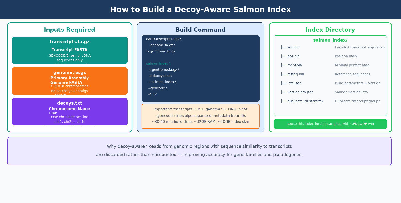
The decoy-aware index requires a single concatenated FASTA (transcripts first, then genome) and a file listing which sequences are the genomic decoys.

# Extract chromosome names from the genome FASTA for the decoys list
grep "^>" GRCh38.primary_assembly.genome.fa.gz \
  | cut -d " " -f 1 \
  | sed 's/>//' \
  > decoys.txt

head -3 decoys.txt
# chr1
# chr2
# chr3

# Concatenate: transcripts MUST come first, genome second
cat gencode.v45.transcripts.fa.gz \
    GRCh38.primary_assembly.genome.fa.gz \
    > gentrome.fa.gz

echo "Gentrome built."

Step 3: Build the Index

salmon index \
  --transcripts references/gentrome.fa.gz \
  --decoys       references/decoys.txt \
  --index        references/salmon_index_hg38_v45 \
  --gencode \
  --threads 12

# --gencode strips the pipe-separated metadata from GENCODE transcript IDs
# e.g. ENST00000456328.2|ENSG00000223972.6|... becomes ENST00000456328.2

Index building for the full human genome takes roughly 30 to 40 minutes on 12 threads and requires around 32GB of RAM. The resulting index directory is about 20GB. This is a one-time cost: the index can be reused across every experiment that uses the same GENCODE release.

How to Run Salmon Quant on Paired-End RNA-Seq

With the index built, quantification runs per sample. For a 30-million-read paired-end library, a single Salmon quant run takes 3 to 5 minutes on 8 threads.

Single Sample

salmon quant \
  --index     references/salmon_index_hg38_v45 \
  --libType   A \
  --mates1    data/raw/sample_ctrl1_R1.fastq.gz \
  --mates2    data/raw/sample_ctrl1_R2.fastq.gz \
  --threads   8 \
  --gcBias \
  --validateMappings \
  --output    results/salmon/sample_ctrl1_quant

Four flags worth understanding:

--libType A tells Salmon to auto-detect strandedness from the data. Salmon will determine whether the library is unstranded (U), stranded forward (SF), or stranded reverse (SR) from the first 100,000 reads. The inferred library type is written to lib_format_counts.json in the output directory. You can also specify it directly: ISR for Illumina TruSeq stranded reverse, ISF for forward stranded.

--gcBias enables GC bias correction. Salmon estimates and corrects for the systematic tendency of GC-rich and GC-poor fragments to be sequenced at different rates. The DESeq2 documentation recommends using the --gcBias flag, which estimates a correction factor for systematic biases commonly present in RNA-seq data, unless you are certain your data do not contain such bias (DESeq2 vignette, Bioconductor).

--validateMappings enables selective alignment, which uses a chaining algorithm to score and validate mapping candidates rather than accepting the first compatible match. This has been the default behavior since Salmon 1.0.0, but specifying it explicitly ensures you get the most accurate results even if default behavior changes.

--seqBias can also be added to model sequence-specific bias (random hexamer priming effects). It adds a small amount of runtime and is worth enabling for datasets with known per-base content biases.

Automating Quantification Across All Samples

For a full experiment, use a bash loop or a simple Python subprocess wrapper:

#!/usr/bin/env bash
# Usage: bash run_salmon.sh data/raw results/salmon

RAW_DIR="${1}"
OUT_DIR="${2:-results/salmon}"
INDEX="references/salmon_index_hg38_v45"
THREADS=8

mkdir -p "${OUT_DIR}"

mapfile -t r1_files < <(find "${RAW_DIR}" -name "*_R1*.fastq.gz" | sort)

echo "Found ${#r1_files[@]} sample(s). Running Salmon quant..."

for r1 in "${r1_files[@]}"; do
    r2="${r1/_R1/_R2}"
    sample=$(basename "${r1}" | sed 's/_R1.*\.fastq\.gz//')

    if [[ ! -f "${r2}" ]]; then
        echo "  WARNING: R2 not found for ${sample}, skipping."
        continue
    fi

    echo "  Quantifying: ${sample}"

    salmon quant \
        --index    "${INDEX}" \
        --libType  A \
        --mates1   "${r1}" \
        --mates2   "${r2}" \
        --threads  "${THREADS}" \
        --gcBias \
        --validateMappings \
        --output   "${OUT_DIR}/${sample}_quant" \
        2>> "${OUT_DIR}/${sample}_salmon.log"

done

echo "All samples complete."

Run it as:

bash run_salmon.sh data/raw results/salmon

Each completed sample produces its own directory under results/salmon/. Once all samples are done, run MultiQC to aggregate the Salmon logs into a single report:

multiqc results/salmon/ \
  --outdir results/multiqc \
  --filename salmon_multiqc_report \
  --force

Understanding the Salmon quant.sf Output File

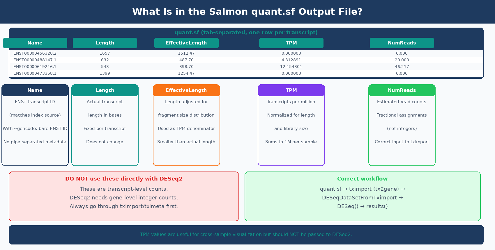
Each sample directory contains a quant.sf file: a tab-separated table with one row per transcript. Here is what each column means:

Name              Length  EffectiveLength  TPM          NumReads
ENST00000456328.2  1657   1512.468         0.000000     0.000
ENST00000488147.1   632    487.697         4.312891    20.000
ENST00000619216.1   543    398.697        12.154301    46.217
ENST00000473358.1  1399   1254.468         0.000000     0.000

Name: the transcript identifier from your reference. With --gencode, this is the bare ENST ID without the pipe-separated metadata suffix.

Length: the actual length of the transcript in bases.

EffectiveLength: the length adjusted for fragment length distribution and positional bias. This is the denominator used in TPM calculation. Shorter fragments can only produce reads from a shorter effective window, so effective length is usually smaller than actual length.

TPM: transcripts per million. The number of reads originating from this transcript per million total reads, after normalization for effective length. TPM values sum to one million across all transcripts in a sample.

NumReads: the estimated number of reads originating from this transcript. These are probabilistic assignments, not integer counts: a read that is compatible with two transcripts contributes fractional counts to each. DESeq2 accepts and handles these fractional estimates correctly by rounding them internally.

Checking Salmon Mapping Rates

Before importing results into R, check that your mapping rates are reasonable. The mapping rate is in the aux_info/meta_info.json file inside each sample directory:

import json
import os
from pathlib import Path

results_dir = Path("results/salmon")
sample_dirs = sorted(results_dir.glob("*_quant"))

print(f"{'Sample':<35} {'Mapped %':>10}")
print("-" * 47)

for sample_dir in sample_dirs:
    meta_path = sample_dir / "aux_info" / "meta_info.json"
    if not meta_path.exists():
        continue
    with open(meta_path) as f:
        meta = json.load(f)

    sample_name = sample_dir.name.replace("_quant", "")
    pct_mapped  = meta.get("percent_mapped", 0.0)

    flag = "  ✓" if pct_mapped >= 75 else "  ⚠ LOW"
    print(f"{sample_name:<35} {pct_mapped:>9.1f}%{flag}")

For a clean poly-A selected human or mouse RNA-seq library mapped to a GENCODE transcriptome, expect 75 to 92 percent mapping. A rate below 70 percent warrants investigation: wrong reference organism, genome-only reads (no cDNA-only reference), strandedness mismatch, or severe degradation are common causes.

MultiQC reads Salmon’s log files directly and surfaces the mapping rate per sample in its General Statistics table, so you rarely need to parse meta_info.json manually. The Python script above is useful when you want to integrate mapping QC into an automated pipeline or flag samples before running R code.

If you are not sure how to interpret the aggregated QC tables and per-sample warnings, Understanding Your QC Report: What FastQC and MultiQC Are Telling You is the companion guide.

How to Import Salmon Output into R with tximeta

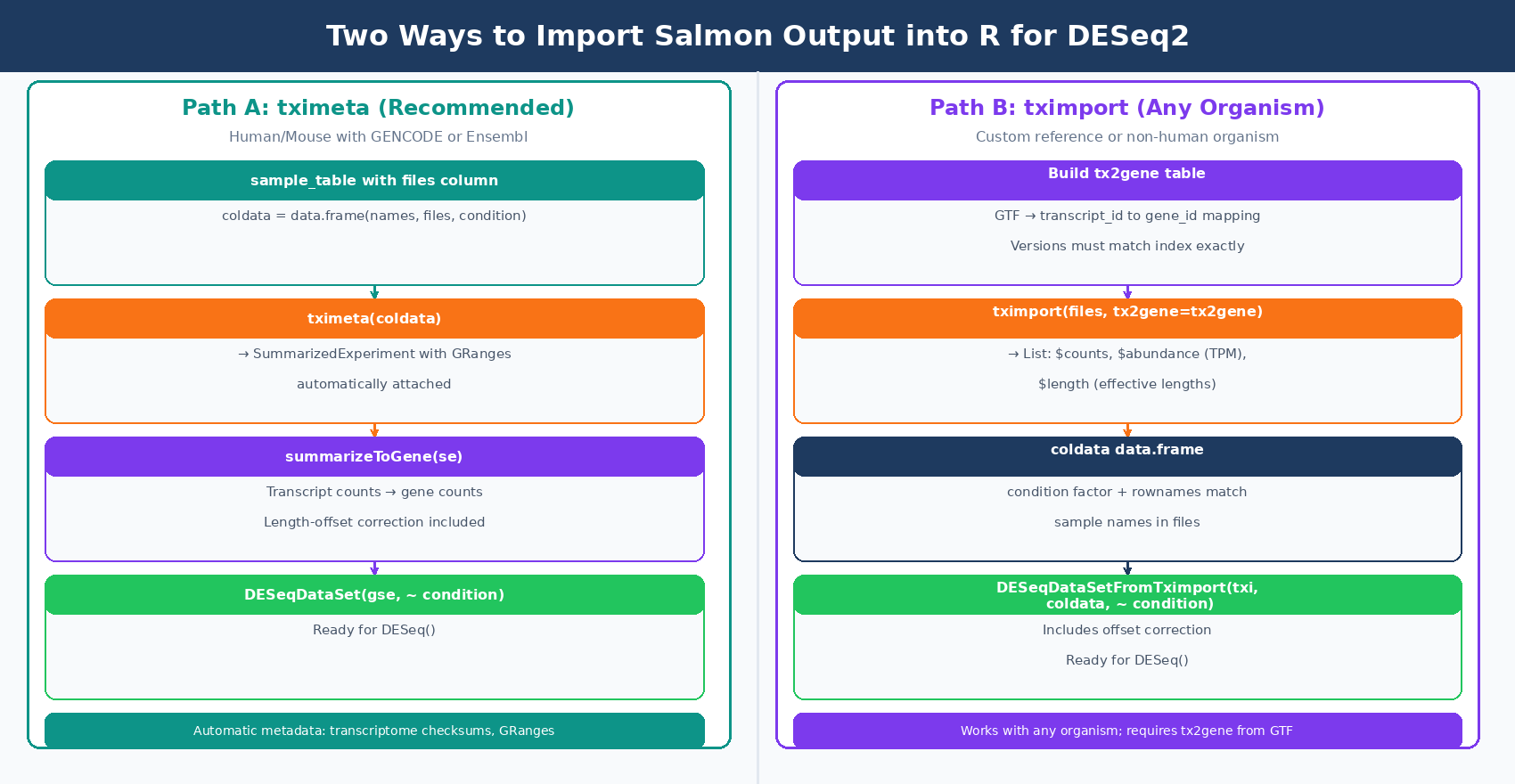
With all samples quantified and QC checked, import the quant.sf files into R. The recommended package is tximeta, which extends tximport by automatically attaching genome coordinate metadata when the transcriptome matches a known source (GENCODE, Ensembl, or RefSeq for human and mouse). Whereas tximport outputs a simple list of matrices, tximeta will output a SummarizedExperiment object with appropriate GRanges added (tximport vignette, Bioconductor).

For projects where tximeta does not recognize the transcriptome (custom references, non-human organisms), tximport is the fallback and works identically for the purposes of DESeq2 input.

Option A: tximeta (Recommended for Human/Mouse with GENCODE or Ensembl)

library(tximeta)
library(DESeq2)

# Build a sample metadata table
# Each row is one sample; 'files' column points to quant.sf
sample_table <- data.frame(
  names     = c("ctrl_1",  "ctrl_2",  "ctrl_3",
                "treat_1", "treat_2", "treat_3"),
  files     = c(
    "results/salmon/ctrl_1_quant/quant.sf",
    "results/salmon/ctrl_2_quant/quant.sf",
    "results/salmon/ctrl_3_quant/quant.sf",
    "results/salmon/treat_1_quant/quant.sf",
    "results/salmon/treat_2_quant/quant.sf",
    "results/salmon/treat_3_quant/quant.sf"
  ),
  condition = factor(c("control", "control", "control",
                       "treated", "treated", "treated"))
)

# Import with tximeta — automatically attaches GRanges metadata
# if transcriptome is from GENCODE, Ensembl, or RefSeq
se <- tximeta(sample_table)

# Summarize from transcript level to gene level
gse <- summarizeToGene(se)

# Build the DESeqDataSet
dds <- DESeqDataSet(gse, design = ~ condition)

# Filter low-count genes before analysis
dds <- dds[rowSums(counts(dds) >= 10) >= 3, ]

dim(dds)
# Typically ~20,000 genes after filtering

Option B: tximport (Works with Any Organism or Custom Reference)

library(tximport)
library(DESeq2)

# Define sample files
sample_names <- c("ctrl_1", "ctrl_2", "ctrl_3",
                  "treat_1", "treat_2", "treat_3")

files <- setNames(
  file.path("results/salmon",
            paste0(sample_names, "_quant"),
            "quant.sf"),
  sample_names
)

# Build the transcript-to-gene mapping from the GTF
# You need this to aggregate transcript counts to gene level
library(GenomicFeatures)

txdb <- makeTxDbFromGFF(
  "references/gencode.v45.annotation.gtf.gz",
  format = "gtf"
)

k       <- keys(txdb, keytype = "TXNAME")
tx2gene <- AnnotationDbi::select(txdb, k, "GENEID", "TXNAME")

# Alternatively, build tx2gene from the GTF with bash:
# zcat references/gencode.v45.annotation.gtf.gz | \
#   awk '$3=="transcript" {split($12,a,"\""); split($10,b,"\""); print a[2]"\t"b[2]}' \
#   > references/tx2gene.tsv

# Import: summarize transcript-level to gene-level
txi <- tximport(
  files,
  type    = "salmon",
  tx2gene = tx2gene
)

# Sample metadata
coldata <- data.frame(
  condition = factor(c("control", "control", "control",
                       "treated", "treated", "treated")),
  row.names = sample_names
)

# Build DESeqDataSet
dds <- DESeqDataSetFromTximport(txi, coldata, ~ condition)
dds <- dds[rowSums(counts(dds) >= 10) >= 3, ]

Validating the Import: Checking Your Count Matrix

Before running DESeq2(), run three quick checks:

# 1. Confirm dimensions look reasonable
dim(dds)
# Rows: ~15,000-22,000 genes after filtering
# Columns: number of samples

# 2. Check library sizes (should be in millions, reasonably balanced)
colSums(counts(dds)) / 1e6
# ctrl_1   ctrl_2   ctrl_3  treat_1  treat_2  treat_3
# 23.1     22.8     21.4     19.7     24.3     22.1

# 3. PCA on variance-stabilized counts to confirm samples cluster by condition
vsd <- vst(dds, blind = TRUE)
plotPCA(vsd, intgroup = "condition")
# Controls should cluster together, treatments separately
# If PC1 separates by batch instead of condition, add batch to the design

A PCA that separates samples by condition rather than by extraction date or library prep run is your final confirmation that the import worked correctly and the experiment is worth proceeding with.

Running the Pipeline Without Writing It Yourself

The full workflow from FASTQ to differential expression, including Salmon quantification with a decoy-aware index, tximeta import, and DESeq2 analysis, is what NotchBio automates end to end. If you want to run this pipeline on your data without building the index, configuring the quant flags, or writing the R import code, upload your FASTQ files at notchbio.app and specify your organism and experimental design. The platform handles indexing, quantification, QC, and DE analysis, and returns the results with all parameters logged for reproducibility.