Understanding Your QC Report: What FastQC and MultiQC Are Telling You
FastQC runs, finishes, and opens an HTML report covered in green ticks, yellow warnings, and red crosses. Most people scan it for red flags, feel vaguely anxious about the yellows, and move on. That approach will get you into trouble specifically because FastQC’s pass/warn/fail thresholds were not designed for RNA-seq. They were calibrated for whole-genome shotgun DNA sequencing, and they will consistently flag RNA-seq data as failing modules where the data is, in fact, perfectly fine.
Understanding what each module is actually measuring, which failures are expected in RNA-seq, and which ones genuinely signal a problem is the difference between spending an afternoon debugging a healthy library and missing real quality issues because everything looked yellow anyway.
This post goes module by module through the FastQC report, then covers what MultiQC adds when you aggregate across samples, and ends with a table that maps every common failure pattern to its probable cause and appropriate action. If you want the hands-on command-line workflow first, read How to Run FastQC and MultiQC on Raw RNA-Seq Reads. If your QC report points to adapter contamination, the next step is usually Trimming Adapters with Trimmomatic and fastp: A Side-by-Side Walkthrough.
The Foundational Rule: FastQC Flags Are for WGS, Not RNA-seq
Before interpreting any individual module, internalize this: FastQC’s thresholds were tuned for a very specific set of assumptions applicable to whole-genome shotgun DNA sequencing. They are less reliable with other types of sequencing including mRNA-Seq, small RNA-Seq, and targeted amplicon sequencing. A “Warn” or “Fail” flag does not mean the sequence run failed. It means the researcher must stop and consider what that result means in the context of that particular sample and sequencing type (MSU RTSF FastQC FAQ).
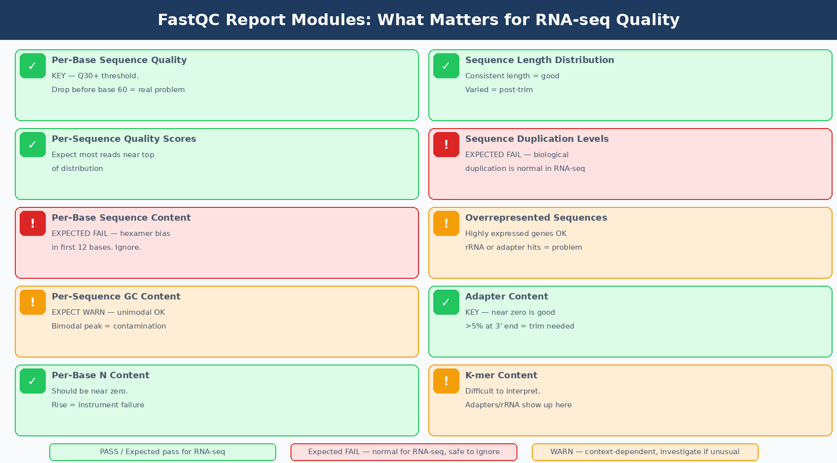
Three modules will almost always fail or warn for perfectly good RNA-seq data:
Per base sequence content fails on RNA-seq because of random hexamer priming bias. The first 10 to 15 bases of every read will show uneven base composition regardless of sample quality, because the random hexamers used during reverse transcription do not bind with equal affinity to all sequences. This is expected, documented, and irrelevant to data quality.
Per sequence GC content warns on RNA-seq because the transcriptome has a GC distribution that differs from a theoretical normal. The shape is usually narrower or shifted compared to a genome-wide expectation. Unless you see a double peak or a dramatic shift, a warning here does not indicate contamination.
Sequence duplication levels flags RNA-seq data as high-duplication because highly expressed transcripts naturally produce many identical reads. A gene expressed at high levels generates the same cDNA fragment repeatedly. This is biology, not PCR artifact. FastQC cannot distinguish the two.
Hold these three in mind before reading any individual report. The flags that actually require attention are elsewhere.
Per-Base Sequence Quality
This is the most important module for assessing raw data quality. For each position across all reads, FastQC shows a boxplot of quality scores. The y-axis is the Phred quality score. The background is divided into three zones: green (Q ≥ 28, very good), yellow (Q 20–28, reasonable), and red (Q < 20, poor).
For Illumina data, expect quality to be high across the full read length, with a characteristic dip in the first 5 to 7 bases and a gradual decline toward the 3-prime end. Read 2 in paired-end sequencing will typically have lower quality than Read 1, which is normal behavior of Illumina chemistry.
What to act on: if the median quality (central line in the boxplot) drops into the orange zone before base 60 on a 100bp read, or if quality collapses sharply, that indicates a real sequencing quality problem. A uniform collapse from the start of the read suggests a run failure. Trimming can recover data with gradual 3-prime quality decay; it cannot fix globally poor quality. For where these QC decisions sit in the broader analysis flow, see Raw Reads to Counts: The Bulk RNA-Seq Pipeline Explained.
A Q30 base calling rate above 80 to 85% across all reads is a reasonable minimum threshold. Modern Illumina instruments running standard RNA-seq libraries routinely achieve Q30 rates of 90% or above.
Per Sequence GC Content
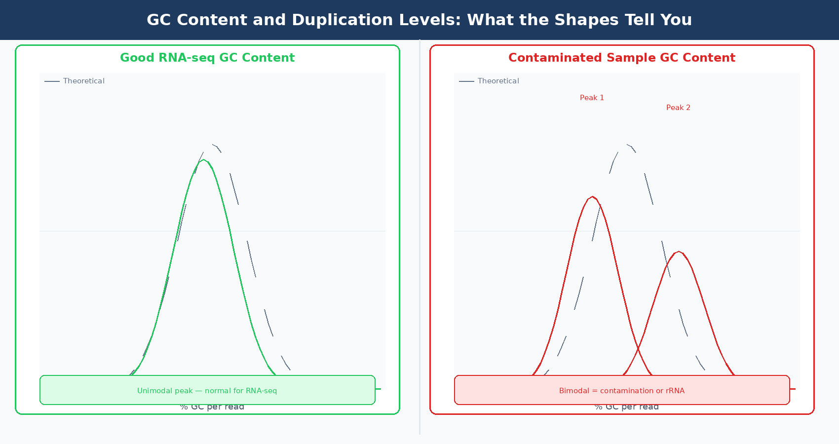
This module plots the GC percentage of each read as a distribution across all reads, and compares it to a theoretical normal distribution built from the observed mean GC content of the data.
For RNA-seq, the distribution should be bell-shaped and centered near your organism’s expected transcriptome GC content. Human transcriptome GC content is roughly 47 to 52%, but the distribution will be narrower than a genome-wide distribution because you are sequencing expressed genes, not the whole genome.
What to investigate: A sharp secondary peak or a shoulder on the distribution is the signal to take seriously. It suggests contamination with another species, ribosomal RNA contamination (which shifts the peak), or a highly overexpressed gene dominating the library. If you see rRNA contamination, the overrepresented sequences module will often confirm it by listing ribosomal sequences.
A shifted peak alone, without secondary peaks, is usually a property of the enrichment strategy. Poly-A selected libraries tend to have slightly different GC profiles from ribo-depleted libraries from the same sample. If all samples in an experiment show the same shift, it is almost certainly a library preparation property rather than a contamination event.
Sequence Duplication Levels
FastQC counts how many sequences appear multiple times in the first 100,000 reads and plots the proportion of reads at each duplication level. There are two lines: the blue line shows the proportion at each duplication level in the full library, the red line shows the proportion that each duplication level would contribute after deduplication.
For whole-genome sequencing, you want most reads to appear once. For RNA-seq, high duplication is expected and does not need to be corrected. A highly expressed gene like ACTB generates enormous numbers of nearly identical cDNA fragments. These are not PCR duplicates; they are genuine expression signal. Removing them would destroy quantification accuracy for your most reliably detected genes.
However, the shape of the duplication curve tells you something about whether the duplication is biological or technical. Biological duplication produces peaks at intermediate duplication levels (sequences appearing 10 to 50 times) concentrated in a few very highly expressed genes. Technical PCR over-amplification tends to elevate duplication uniformly across all sequences, pushing the distribution toward very high duplication levels for many genes, not just the highly expressed ones.
In practice, the most reliable way to assess whether duplication is a problem is to look at your library complexity tools like dupRadar (a Bioconductor package from the nf-core/rnaseq pipeline) or to examine whether your duplication rate is consistent across biological replicates. Libraries with genuine PCR over-amplification tend to have higher and more uniform duplication than their replicates.
Do not deduplicate bulk RNA-seq reads based on FastQC flags
Unlike ChIP-seq or whole-genome sequencing, bulk RNA-seq data should not have reads removed simply because they are duplicates. The tools used for differential expression analysis (DESeq2, edgeR) model biological variation in count data, and removing counts reduces your quantification accuracy for highly expressed genes. Only deduplicate RNA-seq reads if you have specific experimental reasons to do so, such as when using UMI-tagged libraries.
Adapter Content
This module shows the cumulative percentage of reads that contain each of several common Illumina adapter sequences, plotted by read position. The adapter content plot is the primary driver of the trimming decision.
For a well-prepared library with appropriate size selection, adapter content should be near zero or undetectable. Adapters appear in reads only when the cDNA insert is shorter than the read length, causing the sequencer to read through to the adapter on the 3-prime end.
Thresholds that matter for decision-making: Adapter content below 1% across all positions generally does not affect alignment quality, because modern aligners like STAR soft-clip these few bases. Adapter content climbing above 5% in the second half of the read warrants trimming. Content above 10% significantly inflates your unmapped read rate and should be trimmed before alignment.
The shape also matters. A flat plateau at very low levels (< 1%) across the full read length is harmless. A rising curve that begins mid-read and climbs toward the 3-prime end indicates short inserts where the adapters are being read. That is the pattern that requires fastp or Trimmomatic.
Overrepresented Sequences
This module lists sequences that appear in more than 0.1% of the total reads (FastQC raises a warning at this threshold and an error when any sequence exceeds 1% of total reads), checked against the first 200,000 reads in the file. Each overrepresented sequence is compared against a database of known contaminants including adapters and common technical sequences.
For RNA-seq, a small number of overrepresented sequences from highly expressed genes is expected and not concerning. The Harvard HBC Training materials note that for datasets with a highly overexpressed gene, that transcript will register as an overrepresented sequence, and this is “not concerning” in context (Harvard HBC Training).
What is concerning: overrepresented sequences that BLAST to ribosomal RNA, mitochondrial sequences, or adapter/vector sequences. rRNA contamination is the most common culprit in failed poly-A selection steps. If 10% or more of your reads map to rRNA-derived overrepresented sequences, your enrichment step needs troubleshooting.
Per-Base Sequence Content (The Module Most People Misread)
This module plots the proportion of each base (A, T, G, C) at every read position. In WGS data, all four bases should be roughly equal and stable across all positions. In RNA-seq data, the first 10 to 15 bases show a characteristic uneven composition due to random hexamer priming bias during library preparation.
Nearly all RNA-seq libraries will produce a “Fail” flag on this module. This is a known artifact of the library prep chemistry, not a quality problem with your data. The MSU RTSF FastQC FAQ explicitly states: “RNA-Seq data showing this non-uniform base composition will always be classified as Failed by FastQC for this module even though the sequence is perfectly good.”
The specific shape of the bias matters. Random hexamer priming produces a characteristic wavy pattern in the first ~12 bases that then stabilizes. If the instability continues across the full length of the read, or shows a completely different pattern, that could indicate a different issue such as primer contamination.
MultiQC: What It Adds
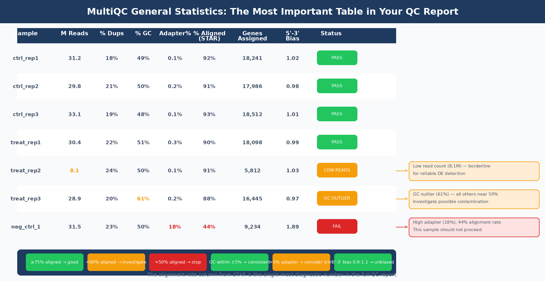
MultiQC aggregates FastQC results across all samples and adds output from downstream pipeline tools — STAR, Salmon, Trimmomatic/fastp, Qualimap, and others. The value it adds over individual FastQC reports is cross-sample comparison: outlier samples become immediately visible when all samples are shown side by side.
The General Statistics table is the first thing to read in any MultiQC report. For a standard RNA-seq pipeline it shows, per sample: total reads, percent GC, percent duplicates, percent adapter content, STAR alignment rate, and the number of reads assigned to genes.
The alignment rate column from STAR is one of the most diagnostically useful numbers in the full QC report. A good quality sample will have at least 75% of reads uniquely mapped. Once values start to drop lower than 60%, it is advisable to start troubleshooting (Harvard HBC Training). Below 50%, alignment failure is severe and the sample should be investigated before including it in downstream analysis.
The STAR alignment bar chart breaks down reads into uniquely mapped, multi-mapped, and unmapped categories. Ideally, uniquely mapped reads dominate and unmapped reads form a small sliver. A large unmapped proportion combined with a low alignment rate is the diagnostic for wrong reference genome, wrong strandedness, contamination, or severely degraded RNA.
The gene body coverage plot from Qualimap or RSeQC shows the depth of coverage across the body of every expressed transcript, from 5-prime to 3-prime. An even, flat line across transcript length indicates unbiased coverage. A curve that rises sharply at the 3-prime end indicates 3-prime bias, the classic signature of RNA degradation. If most of your transcripts show 3-prime bias, your RNA quality was poor even if your RIN scores looked acceptable. The 5-to-3 bias metric reported in the MultiQC table should be close to 1.0 for unbiased data; values approaching 0.5 or 2.0 warrant investigation.
| Module/Metric | What It Measures | Normal for RNA-seq | Action Required If |
|---|---|---|---|
| Per-base quality | Phred score per position | Q30+ across read | Quality drops before base 60 on 100bp reads |
| Per-base sequence content | Base composition per position | Fail in first 12 bases | Instability extends full read length |
| Per-sequence GC content | GC distribution across reads | Warn; narrower peak OK | Bimodal distribution or large shift |
| Sequence duplication | Read duplication rate | High; often 40–70% | Uniform high duplication across all genes |
| Adapter content | Adapter sequences in reads | Near zero | Climbs above 5% in read second half |
| Overrepresented sequences | Sequences >0.1% frequency | Highly expressed genes | Sequences BLAST to rRNA or adapters |
| STAR alignment rate | Uniquely mapped reads | 85–95% | Below 75% (investigate); below 60% (stop) |
| 5’-3’ bias | Gene body coverage uniformity | ~1.0 | Approaches 0.5 or 2.0 |
| GC% between samples | Consistency across samples | Tight cluster | Outlier sample diverges by >5% |
The Diagnostic Decision Tree
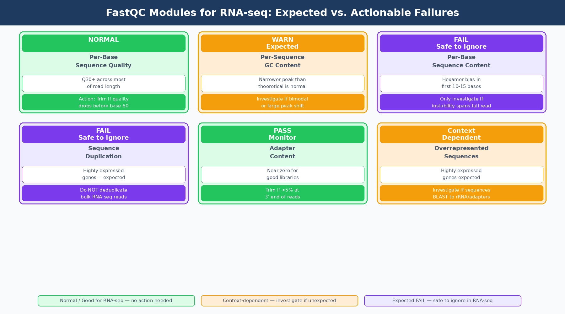
When you see a QC flag or anomalous metric, the question is always: is this expected for RNA-seq, or does it indicate an actual problem? The distinction drives whether you investigate before proceeding or proceed and note the observation.
Expected flags that require no action: per-base sequence content fail in first 15 bases, per-sequence GC content warn with unimodal distribution, sequence duplication warn or fail, per-base N content passing.
Flags to investigate before proceeding: per-base quality below Q28 before the last 10 bases, per-sequence GC content fail with bimodal distribution, overrepresented sequences matching rRNA or adapters at more than 5%, adapter content above 5%.
Hard stops that require root cause analysis: STAR alignment rate below 60%, per-base quality collapse across the full read, more than 20% of reads unmapped in MultiQC bar chart, 5’-3’ bias ratio below 0.5 or above 2.0 in Qualimap output.
Run MultiQC twice — once before trimming and once after alignment
Running MultiQC on pre-trimming FastQC output shows you raw library quality. Running it again after alignment aggregates FastQC, STAR, Qualimap, and Salmon statistics in one report. The two-pass approach lets you see which QC metrics improved after trimming and whether any post-alignment anomalies trace back to something visible in the pre-trimming report.
The QC report is not a quality certificate. It is a diagnostic tool. Reading it well means knowing which modules to ignore for your data type, which patterns indicate genuine problems, and which single number (the STAR alignment rate) summarizes overall sample health better than any individual FastQC module flag. Before your DESeq2 analysis runs, every sample should have a documented alignment rate above 75% and a per-base quality score above Q28 for the bulk of its read length. If it does not, the analysis results from that sample are unreliable regardless of how they look downstream.
NotchBio includes a full QC report with every pipeline run, aggregating FastQC, STAR alignment statistics, and Qualimap gene body coverage metrics in a single view. Samples with anomalous alignment rates or 3-prime bias are automatically flagged before the differential expression analysis proceeds. You can explore the QC dashboard at notchbio.app.
Further reading
Read another related post
Trimming Adapters with Trimmomatic and fastp: A Side-by-Side Walkthrough
When adapter trimming helps, when it hurts, and how to run Trimmomatic and fastp on RNA-seq data with the parameter choices that actually matter.
TutorialHow to Run FastQC and MultiQC on Raw RNA-Seq Reads
A hands-on guide to automating RNA-seq QC across dozens of samples using FastQC and MultiQC, with bash and Python scripts for parsing and flagging failures.
Research GuideRaw Reads to Counts: The Bulk RNA-Seq Pipeline Explained
A practical breakdown of every computational step in bulk RNA-seq: from FASTQ quality control through trimming, alignment, and quantification to your final count matrix.