Tutorial

Importing Salmon Output into R: tximeta, tximport, and DESeq2 Setup

By Abdullah Shahid · April 14, 2026 · 16 min read

rna-seq tutorial differential-expression

Salmon has finished running. You have a directory full of quant.sf files. The next step sounds simple: import them into R and hand them to DESeq2. In practice, this step breaks more often than any other in the bulk RNA-seq pipeline, almost always because of a transcript ID mismatch between the Salmon output and the annotation table used to map transcripts to genes.

This tutorial walks through the full import workflow in R: understanding the difference between tximeta and tximport, building and validating a tx2gene mapping table, diagnosing and fixing the most common ID mismatch errors, setting up multi-factor designs, and validating your count matrix before running differential expression analysis.

If you have not generated the quant.sf files yet, start with How to Quantify RNA-Seq Reads with Salmon. If you want the downstream model after import, How to Run DESeq2: A Complete Walkthrough from Count Matrix to Results is the next step.

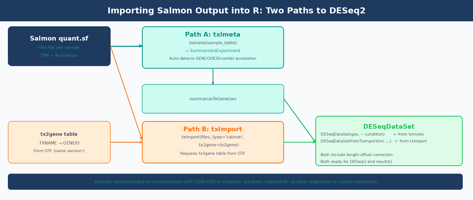
R workflow diagram showing Salmon quant.sf files being imported via tximeta or tximport, with tx2gene mapping table, producing a DESeqDataSet ready for DESeq2 analysis — Figure 1: The import pipeline from Salmon quant.sf files to a DESeqDataSet. tximeta handles annotation automatically for recognized transcriptomes. tximport requires a tx2gene table you provide but works with any organism or custom reference.

tximeta vs tximport: What Is the Difference?

Both packages do the same core job: read quant.sf files, aggregate transcript-level counts to gene-level counts, apply a length-offset correction for isoform usage bias, and return a structure that DESeq2 can consume. The difference is in what extra work each one does for you.

tximport (Soneson, Love, and Robinson, 2015) is the lower-level package. It returns a named list with three matrices: $counts (gene-level estimated counts), $abundance (TPM values), and $length (effective gene lengths). You are responsible for providing a tx2gene data frame that maps transcript IDs to gene IDs. You are also responsible for making sure those IDs match what is in your quant.sf files. When they do not match, you get the most common tximport error: None of the transcripts in the quantification files are present in the first column of tx2gene.

tximeta (Love et al., 2020) extends tximport by automatically resolving the transcript annotation when the transcriptome matches a known source: GENCODE, Ensembl, or RefSeq for human and mouse. It computes a checksum of the Salmon index and looks up matching annotation metadata from a pre-built database. Instead of a list of matrices, it returns a SummarizedExperiment object with gene coordinates, genome ranges, and provenance metadata already attached. You then call summarizeToGene() to aggregate to gene level. The DESeqDataSet() function accepts this directly.

The practical implication: if you used GENCODE or Ensembl for human or mouse, use tximeta. You get automatic metadata and skip the tx2gene table entirely. For any other organism, any custom transcriptome, or any situation where tximeta fails to recognize your index, use tximport with a manually built tx2gene table.

The DESeq2 recommended pipeline starts with tximport or tximeta

The DESeq2 vignette states explicitly: “Our recommended pipeline for DESeq2 is to use fast transcript abundance quantifiers upstream of DESeq2, and then to create gene-level count matrices using tximport.” This is not just a convenience: the tximport pipeline applies a length-offset correction that accounts for potential changes in average transcript length across samples from differential isoform usage, which a plain count matrix does not capture (DESeq2 vignette, Bioconductor).

Installing the Required Packages

if (!requireNamespace("BiocManager", quietly = TRUE))
    install.packages("BiocManager")

BiocManager::install(c(
    "tximeta",       # recommended import package
    "tximport",      # fallback for custom transcriptomes
    "DESeq2",        # differential expression
    "GenomicFeatures", # for building tx2gene from GTF
    "AnnotationDbi", # for database queries
    "rtracklayer"    # for importing GTF as GRanges
))

Path A: Importing with tximeta (GENCODE or Ensembl, Human or Mouse)

If you used GENCODE or Ensembl to build your Salmon index, tximeta is the cleanest import path. It automatically detects the transcriptome from the Salmon index digest stored inside your quant directory, attaches the relevant annotation, and produces a fully-annotated SummarizedExperiment.

Step 1: Build the Sample Table

tximeta requires a data frame with at least two columns: files (the path to each quant.sf) and names (the sample identifier). Any additional columns become sample metadata.

library(tximeta)
library(DESeq2)

# Build the sample table
# Every column beyond 'files' and 'names' becomes colData in the SummarizedExperiment
sample_table <- data.frame(
    names     = c("ctrl_1",  "ctrl_2",  "ctrl_3",
                  "treat_1", "treat_2", "treat_3"),
    files     = c(
        "results/salmon/ctrl_1_quant/quant.sf",
        "results/salmon/ctrl_2_quant/quant.sf",
        "results/salmon/ctrl_3_quant/quant.sf",
        "results/salmon/treat_1_quant/quant.sf",
        "results/salmon/treat_2_quant/quant.sf",
        "results/salmon/treat_3_quant/quant.sf"
    ),
    condition = factor(c("control", "control", "control",
                         "treated", "treated", "treated"),
                       levels = c("control", "treated"))
)

# Verify all files exist before importing
stopifnot(all(file.exists(sample_table$files)))

Step 2: Import with tximeta

# Import: tximeta resolves annotation automatically from the Salmon index digest
se <- tximeta(sample_table)

# What you get back:
class(se)
# [1] "RangedSummarizedExperiment"
# attr(,"package")
# [1] "SummarizedExperiment"

# Check dimensions (transcript level at this point)
dim(se)
# [1] 247627      6   (transcripts x samples, for human GENCODE v45)

If tximeta recognizes the transcriptome, you will see messages like found matching transcriptome and metadata will be populated automatically. If it does not recognize the transcriptome, it returns an unranged SummarizedExperiment without coordinates, which still works for DESeq2 but without the genome annotation benefit.

Step 3: Summarize to Gene Level

# Aggregate from transcript level to gene level
gse <- summarizeToGene(se)

dim(gse)
# [1] 62703     6   (genes x samples)

# Check that gene IDs look correct
head(rownames(gse))
# [1] "ENSG00000223972.6" "ENSG00000227232.5" "ENSG00000278267.1"
# [4] "ENSG00000243485.5" "ENSG00000284332.1" "ENSG00000237613.2"

Step 4: Build the DESeqDataSet

# Build DESeqDataSet from the gene-level SummarizedExperiment
dds <- DESeqDataSet(gse, design = ~ condition)

# Filter low-count genes
# Keep genes with at least 10 counts in at least 3 samples
keep <- rowSums(counts(dds) >= 10) >= 3
dds  <- dds[keep, ]

dim(dds)
# Typically ~15,000-20,000 genes remaining after filtering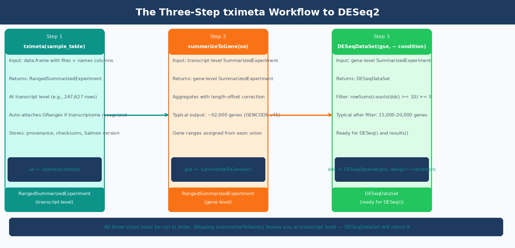

Code flow diagram showing tximeta() producing a transcript-level SummarizedExperiment, summarizeToGene() collapsing to gene level with GRanges metadata, and DESeqDataSet() producing the DESeq2 input object, with the key output objects labeled at each step — Figure 2: The three-step tximeta workflow. tximeta returns a transcript-level SummarizedExperiment; summarizeToGene aggregates to gene level; DESeqDataSet wraps the result with a design formula for DESeq2.

Path B: Importing with tximport and a tx2gene Table

For any organism other than human or mouse, any custom reference, or when tximeta does not recognize your transcriptome, you need tximport with a manually built tx2gene mapping table.

What Is a tx2gene Table?

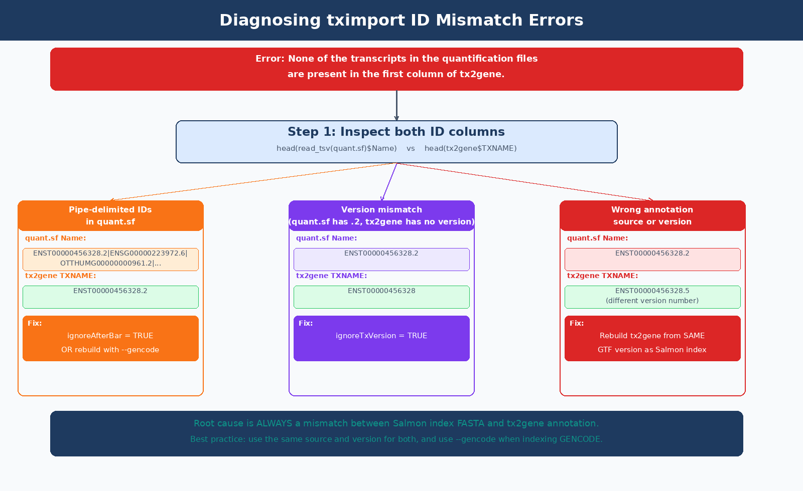
A tx2gene table is a two-column data frame mapping transcript IDs (column 1) to gene IDs (column 2). The column names do not matter but the order does: transcript first, gene second. The transcript IDs must match exactly what appears in the Name column of your quant.sf files.

This is where most errors happen. If you built your Salmon index from GENCODE transcripts without the --gencode flag, your quant.sf Name column contains the full pipe-delimited GENCODE header like ENST00000456328.2|ENSG00000223972.6|OTTHUMG00000000961.2|.... If your tx2gene table contains bare ENST00000456328.2 IDs, tximport will report None of the transcripts in the quantification files are present in the first column of tx2gene and return nothing useful.

Building the tx2gene Table from a GTF

The safest way to build tx2gene is from the same GTF file that corresponds to your Salmon index transcriptome. This guarantees ID format compatibility.

Method 1: Using GenomicFeatures (recommended, works with any GTF)

library(GenomicFeatures)
library(AnnotationDbi)

# Build a TxDb object from the GTF
# Use the same GTF version that was used to build your Salmon index
txdb <- makeTxDbFromGFF(
    "references/gencode.v45.annotation.gtf.gz",
    format   = "gtf",
    organism = "Homo sapiens"
)

# Extract transcript-to-gene mapping
k       <- keys(txdb, keytype = "TXNAME")
tx2gene <- AnnotationDbi::select(
    txdb,
    keys     = k,
    columns  = "GENEID",
    keytype  = "TXNAME"
)

# Result: two-column data frame
head(tx2gene)
#             TXNAME           GENEID
# 1 ENST00000456328.2 ENSG00000223972.6
# 2 ENST00000450305.2 ENSG00000223972.6
# 3 ENST00000473358.1 ENSG00000243485.5

dim(tx2gene)
# [1] 247627      2

Method 2: From the GTF using bash (fast, no R dependencies for this step)

# Extract transcript_id and gene_id from GTF in one command
# Works for both GENCODE and Ensembl GTFs
zcat references/gencode.v45.annotation.gtf.gz \
  | awk '$3 == "transcript"' \
  | grep -oP 'transcript_id "[^"]+"|gene_id "[^"]+"' \
  | paste - - \
  | awk '{gsub(/transcript_id "|gene_id "|"/,""); print $1"\t"$2}' \
  > references/tx2gene_v45.tsv

# Then load in R:
# tx2gene <- read.table("references/tx2gene_v45.tsv",
#                       col.names = c("TXNAME", "GENEID"))

Verifying That Your IDs Match

Before running tximport, check that the IDs in your tx2gene table match the IDs in your quant.sf files:

library(tximport)
library(readr)

# Peek at the Name column of one quant.sf file
sample_ids <- read_tsv(
    "results/salmon/ctrl_1_quant/quant.sf",
    n_max  = 5,
    col_types = cols_only(Name = col_character())
)
cat("IDs in quant.sf:\n")
print(sample_ids$Name)
# ENST00000456328.2
# ENST00000450305.2
# ENST00000473358.1

cat("\nIDs in tx2gene:\n")
print(head(tx2gene$TXNAME))
# ENST00000456328.2
# ENST00000450305.2

# Check for overlap
overlap <- mean(sample_ids$Name %in% tx2gene$TXNAME)
cat(sprintf("%.0f%% of quant.sf IDs found in tx2gene\n", overlap * 100))
# 100% of quant.sf IDs found in tx2gene  <- what you want

If overlap is zero or near zero, you have an ID mismatch. The section below covers how to diagnose and fix it.

Running tximport

# Build file paths
sample_names <- c("ctrl_1",  "ctrl_2",  "ctrl_3",
                  "treat_1", "treat_2", "treat_3")

files <- setNames(
    file.path("results/salmon",
              paste0(sample_names, "_quant"),
              "quant.sf"),
    sample_names
)

stopifnot(all(file.exists(files)))

# Import and summarize to gene level
txi <- tximport(
    files,
    type    = "salmon",
    tx2gene = tx2gene
)

# What you get back:
names(txi)
# [1] "abundance"            "counts"               "length"
# [4] "countsFromAbundance"

# abundance = TPM matrix (genes x samples)
# counts    = estimated count matrix (genes x samples, may be fractional)
# length    = effective gene length matrix (genes x samples)

dim(txi$counts)
# [1] 62703     6

# Fractional counts from probabilistic assignment are expected
head(round(txi$counts[, 1], 3))
#      ENSG00000223972.6  ENSG00000243485.5  ENSG00000238009.6
#                  0.000              0.000           0.000

Building the DESeqDataSet from tximport

# Sample metadata
coldata <- data.frame(
    condition = factor(c("control", "control", "control",
                         "treated", "treated", "treated"),
                       levels = c("control", "treated")),
    row.names = sample_names
)

# The DESeqDataSetFromTximport function handles the length offset correctly
dds <- DESeqDataSetFromTximport(
    txi,
    colData = coldata,
    design  = ~ condition
)

# Filter low counts
keep <- rowSums(counts(dds) >= 10) >= 3
dds  <- dds[keep, ]

Do not use DESeqDataSetFromMatrix with txi$counts directly

Using DESeqDataSetFromMatrix(countData = txi$counts, ...) skips the length-offset correction that tximport computes. The offset corrects for differential isoform usage across samples, which can alter apparent gene length and bias your results. Always use DESeqDataSetFromTximport(txi, ...) so the offset is included. The only exception is 3-prime tagged RNA-seq data (QuantSeq), where length bias is absent by design (tximport vignette).

How to Fix the Most Common tximport ID Mismatch Errors

The error None of the transcripts in the quantification files are present in the first column of tx2gene has three common causes:

Cause	How to Diagnose	Fix
Built Salmon index without `--gencode` flag	quant.sf Name column has full pipe-delimited GENCODE header	Rebuild index with `--gencode`, or use `ignoreAfterBar = TRUE` in tximport
tx2gene from wrong annotation version	ENST version numbers differ (e.g., `.2` vs `.5`)	Rebuild tx2gene from same GTF version used in index
Ensembl index but GENCODE tx2gene (or vice versa)	quant.sf has `ENST00000456328.2`, tx2gene has `ENST00000456328`	Use `ignoreTxVersion = TRUE`, or rebuild from matching source
tx2gene columns are in wrong order	Gene column is first instead of transcript	Swap columns: `tx2gene <- tx2gene[, c("TXNAME", "GENEID")]`

Fix 1: GENCODE Pipe-Delimited Names (ignoreAfterBar)

If you built your Salmon index from a GENCODE FASTA without using --gencode, your quant.sf Name column looks like:

ENST00000456328.2|ENSG00000223972.6|OTTHUMG00000000961.2|...|DDX11L2|1657|processed_transcript|

The ignoreAfterBar = TRUE argument strips everything after the first |:

txi <- tximport(
    files,
    type           = "salmon",
    tx2gene        = tx2gene,
    ignoreAfterBar = TRUE   # strips pipe-delimited suffix from quant.sf IDs
)

The cleaner fix is to rebuild the Salmon index with --gencode, which strips the pipe-delimited metadata at index build time and gives you bare ENST IDs in your quant.sf files going forward.

Fix 2: Version Number Mismatches (ignoreTxVersion)

If your quant.sf IDs have version suffixes (e.g., ENST00000456328.2) but your tx2gene table has unversioned IDs (e.g., ENST00000456328), use ignoreTxVersion = TRUE:

txi <- tximport(
    files,
    type             = "salmon",
    tx2gene          = tx2gene,
    ignoreTxVersion  = TRUE   # strips ".2" suffix from ENST IDs in quant.sf
)

Important: do not use ignoreTxVersion when both files already have matching versions. The flag strips version suffixes from the quant.sf IDs only, not from tx2gene. If both have versions and they match, using the flag may cause unintended stripping and re-introduce mismatches. Use it only when there is a documented version format difference between the two.

ignoreTxVersion and ignoreAfterBar are rescue flags, not defaults

These flags exist to handle specific mismatch scenarios. The correct solution is always to ensure your Salmon index FASTA and your tx2gene annotation come from the same source and the same release. Using these flags when IDs already match correctly does nothing harmful, but it can mask a deeper configuration problem if the mismatch is not what you think it is.

Diagnosis flowchart for the tximport error 'None of the transcripts in the quantification files are present in the first column of tx2gene', showing how to inspect quant.sf Name column and tx2gene TXNAME column, identify the mismatch type, and apply the correct fix — Figure 3: Diagnosing ID mismatch errors in tximport. Always inspect both the quant.sf Name column and the tx2gene TXNAME column before applying any fix. The root cause is always a format or version difference between your Salmon index transcriptome and your annotation source.

Setting Up Multi-Factor Designs

Most real experiments have more than one explanatory variable. A paired design, a batch variable, or a multi-condition experiment all require a design formula that captures the full structure of the data.

This is the same design-formula decision discussed in Batch Effects: The Silent Killer of RNA-Seq Studies, and the same structure you will see visually in PCA and Clustering for RNA-Seq QC in Python.

Two-Factor Design with Batch

# Sample table with two factors
coldata_batch <- data.frame(
    condition = factor(c("control", "control", "control",
                         "treated", "treated", "treated"),
                       levels = c("control", "treated")),
    batch     = factor(c("batch_A", "batch_A", "batch_B",
                         "batch_A", "batch_A", "batch_B")),
    row.names = sample_names
)

# Include batch as a blocking factor in the design
# ~ batch + condition tests for condition effect
# after accounting for batch variance
dds_batch <- DESeqDataSetFromTximport(
    txi,
    colData = coldata_batch,
    design  = ~ batch + condition
)

keep <- rowSums(counts(dds_batch) >= 10) >= 3
dds_batch <- dds_batch[keep, ]

Paired Design (Before/After, Matched Samples)

# Paired design: same patient before and after treatment
coldata_paired <- data.frame(
    patient   = factor(c("P1", "P2", "P3", "P1", "P2", "P3")),
    condition = factor(c("before", "before", "before",
                         "after",  "after",  "after"),
                       levels = c("before", "after")),
    row.names = sample_names
)

# Include patient as blocking factor
# This removes inter-patient variance from the residual,
# dramatically increasing power to detect the treatment effect
dds_paired <- DESeqDataSetFromTximport(
    txi,
    colData = coldata_paired,
    design  = ~ patient + condition
)

Multi-Condition Design

# Three conditions: control, dose_low, dose_high
coldata_multi <- data.frame(
    condition = factor(
        c("control",  "control",  "control",
          "dose_low", "dose_low", "dose_high"),
        levels = c("control", "dose_low", "dose_high")
    ),
    row.names = sample_names
)

dds_multi <- DESeqDataSetFromTximport(
    txi,
    colData = coldata_multi,
    design  = ~ condition
)

# With multiple conditions, results() uses contrasts to specify which comparison:
# dds_multi <- DESeq(dds_multi)
# res_low_vs_ctrl  <- results(dds_multi, contrast = c("condition", "dose_low",  "control"))
# res_high_vs_ctrl <- results(dds_multi, contrast = c("condition", "dose_high", "control"))

Validating the Count Matrix Before Running DESeq2

Running a few diagnostics on the DESeqDataSet before calling DESeq() catches problems while they are still fixable.

# 1. Check library sizes (total counts per sample)
# Large imbalances are handled by DESeq2 normalization
# but very low-count samples may lack sensitivity
lib_sizes <- colSums(counts(dds)) / 1e6
cat("Library sizes (millions of reads):\n")
print(round(lib_sizes, 1))
# ctrl_1  ctrl_2  ctrl_3  treat_1 treat_2 treat_3
#   22.4    19.8    23.1    21.0    24.5    20.9
# Flag samples below 10M reads

# 2. PCA on variance-stabilized counts to check sample clustering
vsd <- vst(dds, blind = TRUE)
plotPCA(vsd, intgroup = "condition")
# Expect: samples cluster by condition, not by extraction date
# If PC1 separates by batch instead, add batch to the design formula

# 3. Sample distance heatmap
library(pheatmap)
sampleDists <- dist(t(assay(vsd)))
pheatmap(
    as.matrix(sampleDists),
    clustering_distance_rows = sampleDists,
    clustering_distance_cols = sampleDists,
    main = "Sample-to-sample distances (VST)"
)
# Replicates should cluster together; outliers appear as distant rows

# 4. Check that the reference level is set correctly
levels(dds$condition)
# [1] "control" "treated"   <- control is reference (first level)
# If not:
# dds$condition <- relevel(dds$condition, ref = "control")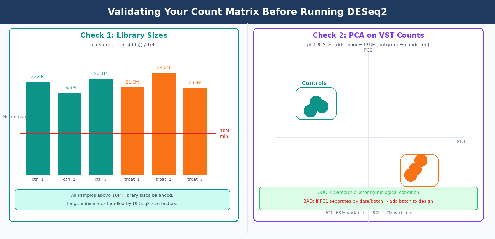

Two diagnostic plots: left shows a bar chart of library sizes per sample in millions of reads with a dashed line at 10M as the minimum recommended threshold; right shows a PCA plot of variance-stabilized counts with samples colored by condition and correctly clustering by biological condition rather than technical batch — Figure 4: Two mandatory checks before running DESeq2. Library sizes below 10M reads warrant flagging. PCA should cluster samples by biological condition. If PC1 separates by batch, add batch to the design formula before proceeding.

Running DESeq2

With the DESeqDataSet validated, the analysis runs in two lines:

# Run differential expression analysis
dds <- DESeq(dds)

# Extract results (default: last variable in design, last vs first level)
res <- results(dds)

# Summary of significant genes
summary(res)
# out of 18,234 with nonzero total read count
# adjusted p-value < 0.1:
# LFC > 0 (up)       : 412, 2.3%
# LFC < 0 (down)     : 388, 2.1%

# Apply LFC shrinkage for visualization (recommended)
res_shrunk <- lfcShrink(dds,
                         coef  = "condition_treated_vs_control",
                         type  = "apeglm")

# Save results
write.csv(as.data.frame(res_shrunk),
          file = "results/deseq2_treated_vs_control.csv")

The lfcShrink step applies adaptive shrinkage to log2 fold changes, pulling noisy estimates from lowly expressed genes toward zero. It does not change which genes are significant; it makes MA plots and volcano plots more interpretable by reducing the scatter from high-variance, low-count genes.

NotchBio automates this full pipeline from Salmon output to DESeq2 results, including the tximeta import, multi-factor design validation, and LFC shrinkage. If you prefer to skip the R setup and focus on interpreting results, upload your quant.sf files and sample metadata at notchbio.app.

Read another related post

View all posts