How to Run DESeq2 in R: From Salmon Counts to DEG Results
Getting a list of differentially expressed genes from DESeq2 is not the hard part. Getting a list you can actually trust is.
Most DESeq2 errors are quiet. The pipeline runs cleanly, you get thousands of genes, and none of it flags an error. But if you fed it normalized counts instead of raw counts, set your reference level wrong, or forgot to include batch in the design formula, your results are biased and you have no warning.
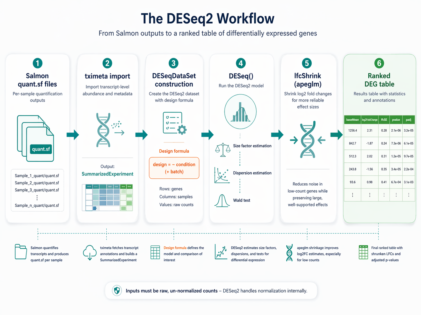
This tutorial walks through the full DESeq2 workflow in R: importing Salmon quant.sf files with tximeta, building the DESeqDataSet, running the model, applying apeglm shrinkage, and exporting a clean ranked results table. We use the r-rnaseq conda environment from the Ubuntu and macOS setup guide. Your Salmon outputs live in results/quant/ from the Salmon indexing and quantification tutorial.
Why Raw Counts Matter More Than You Think
DESeq2 expects raw, un-normalized integer counts. This is not a preference. It is a requirement for the statistical model to work correctly.
The negative binomial model that DESeq2 uses requires knowledge of the raw count variance. If you pre-normalize your data before passing it to DESeq2, the model cannot accurately estimate dispersion, and your p-values will be wrong. Do not provide TPM, RPKM, or CPM to DESeq2.
It is important to not provide counts that were pre-normalized for sequencing depth, as the statistical model is most powerful when applied to un-normalized counts and is designed to account for library size differences internally.
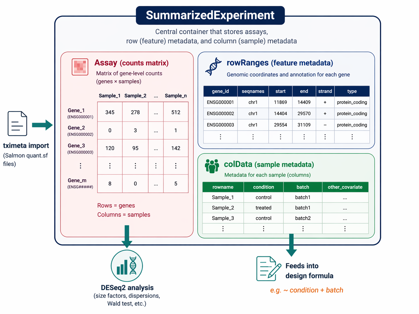
The tximeta import pipeline handles this correctly. It converts Salmon’s estimated transcript-level abundances into gene-level counts using the offsets method, which accounts for differences in transcript length across samples. The resulting counts are appropriate for DESeq2 without any further transformation.
How to Import Salmon quant.sf Files with tximeta
Activate the R environment and open an R session or RStudio.
# Activate from terminal:# conda activate r-rnaseq
library(tximeta)library(DESeq2)library(dplyr)library(readr)
Build the sample table
The sample table maps each Salmon output directory to its metadata. Every column you want available in the design formula must be present here.
# List all quant directoriesquant_dirs <- list.dirs("results/quant", recursive = FALSE, full.names = TRUE)
# Parse sample names from directory names# Assumes directories are named like: SRR26891234_quantsample_names <- sub("_quant$", "", basename(quant_dirs))
# Load sample metadata (from pysradb output in the GEO/SRA download step)metadata <- read_csv("sample_sheet.csv") |>  filter(sample_id %in% sample_names) |>  arrange(match(sample_id, sample_names))
# Build the coldata table for tximetacoldata <- data.frame(  names      = sample_names,  files      = file.path(quant_dirs, "quant.sf"),  condition  = factor(metadata$condition),  batch      = factor(metadata$batch),     # include if present  row.names  = sample_names)
# Set the reference level BEFORE building the DESeqDataSet# The reference level is your control conditioncoldata$condition <- relevel(coldata$condition, ref = "control")
# Verify all quant.sf files existstopifnot(all(file.exists(coldata$files)))cat("All quant.sf files found:", nrow(coldata), "samples\n")
Import with tximeta
# tximeta automatically fetches GENCODE/Ensembl transcript annotations# It attaches genomic ranges to the SummarizedExperimentse <- tximeta(coldata)
# Summarize transcript-level estimates to gene level# The tx2gene mapping is built automatically from the metadata in segse <- summarizeToGene(se)
cat("Gene-level SummarizedExperiment dimensions:", dim(gse), "\n")# Should show ~62,000 genes x 12 samples for GENCODE v47
tximeta vs tximport: which one to use
Use tximeta if you quantified with GENCODE or Ensembl references. It auto-fetches the tx2gene mapping and attaches genomic coordinates. Use tximport if you used a custom reference or if tximeta fails to recognize your index. The downstream DESeq2 code is identical either way.
How to Build a DESeqDataSet with the Right Design Formula
The design formula is the most consequential decision in the analysis. It tells DESeq2 which variables to model and which comparison to make.
# Simple two-group design: condition onlydds <- DESeqDataSet(gse, design = ~ condition)
# If you have a batch effect that MultiQC confirmed (from the QC step)# Add batch to the design to control for it# dds <- DESeqDataSet(gse, design = ~ batch + condition)
The order of terms in the formula matters. DESeq2 tests the last term. With ~ batch + condition, it controls for batch and tests condition. With ~ condition + batch, it would test batch instead.
Filter low-count genes
Genes with very low counts across all samples add noise and reduce statistical power by increasing the multiple testing burden. Filter them before running the model.
# Keep genes with at least 10 counts in at least 3 samples# The 3 here should match your smallest group sizekeep <- rowSums(counts(dds) >= 10) >= 3dds  <- dds[keep, ]
cat("Genes retained after filtering:", nrow(dds), "\n")# Typically 18,000 to 22,000 protein-coding genes for human
Set your reference level before running DESeq()
DESeq2 computes fold changes as treated vs reference. If you do not call relevel() before constructing the DESeqDataSet, R defaults to alphabetical ordering. Your fold changes will be correct in magnitude but potentially in the wrong direction. Set the reference level explicitly and confirm it with levels(dds$condition)[1].
How to Run DESeq() and Interpret Each Step
The single DESeq() call runs three sequential steps internally: size factor estimation, dispersion estimation, and the Wald test.
# This takes 2-10 minutes depending on dataset sizedds <- DESeq(dds)DESeq2 prints progress as it runs.
estimating size factorsestimating dispersionsgene-wise dispersion estimatesmean-dispersion relationshipfinal dispersion estimatesfitting model and testingEach step matters. Size factor estimation corrects for library depth differences between samples. Dispersion estimation models the gene-level variance, which is what makes the Wald test conservative enough to control false discoveries in RNA-seq data.
Extract results for the contrast of interest
# Extract results for the condition comparisonres <- results(  dds,  name     = "condition_treated_vs_control",  alpha    = 0.05     # FDR threshold for independent filtering)
# Summary of resultssummary(res)
The summary() output looks like:
out of 19,847 with nonzero total read countadjusted p-value < 0.05LFC > 0 (up) : 1,243, 6.3%LFC < 0 (down) : 987, 5.0%outliers [1] : 23, 0.12%low counts [2] : 2,104, 10.6%How to Apply apeglm LFC Shrinkage
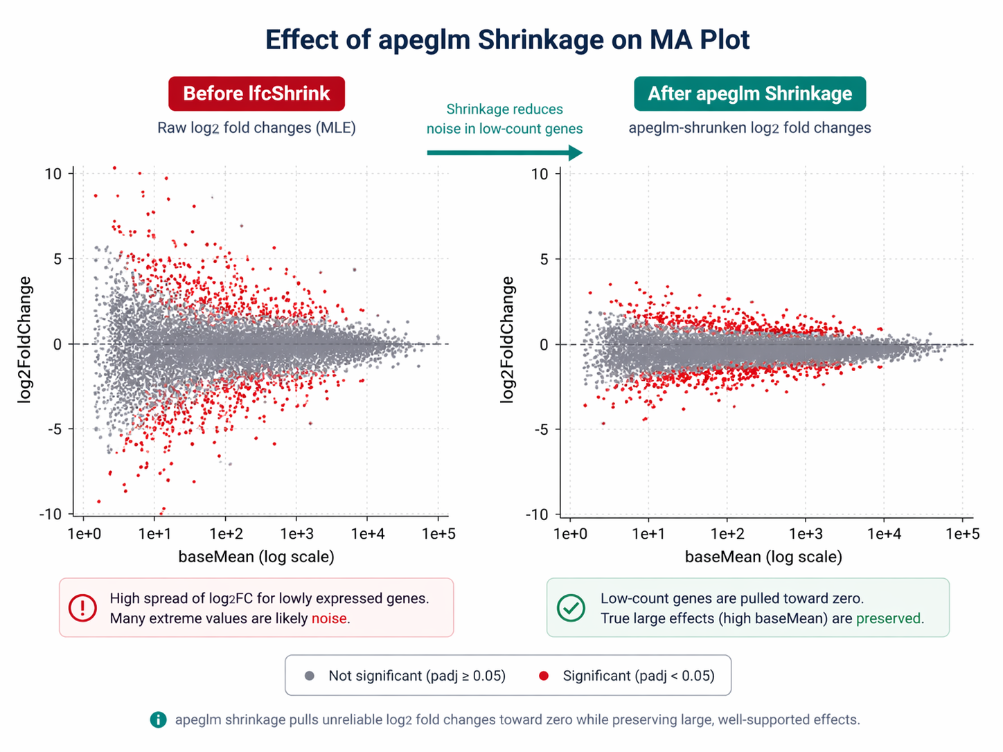
Raw log2 fold changes from DESeq2 are maximum likelihood estimates. Genes with low counts will have extreme fold changes with very high uncertainty. These noisy estimates make volcano plots uninformative and mislead gene ranking.
lfcShrink with apeglm applies a Bayesian shrinkage estimator that pulls unreliable fold changes toward zero while preserving large, well-supported fold changes. apeglm and ashr shrinkage methods help to preserve the size of large LFC and can be used to compute s-values. These properties are related to wide-tailed priors that avoid shrinking large LFCs.
library(apeglm)
# Get the coefficient name to shrinkresultsNames(dds)# [1] "Intercept" "condition_treated_vs_control"
# Apply apeglm shrinkageres_shrunk <- lfcShrink(  dds,  coef = "condition_treated_vs_control",  type = "apeglm")
# Compare before vs after shrinkage for a low-count gene# Raw LFC for a gene with baseMean = 4: might show log2FC = 8.3# Shrunken LFC for same gene: pulled toward ~1.2
Use the shrunken results for visualization and ranking. Use the unshrunken results only if you need p-values with specific numeric contrast weights.
How to Annotate Results with Gene Symbols
DESeq2 works with Ensembl gene IDs by default. Convert them to gene symbols before exporting.
library(AnnotationDbi)library(org.Hs.eg.db)
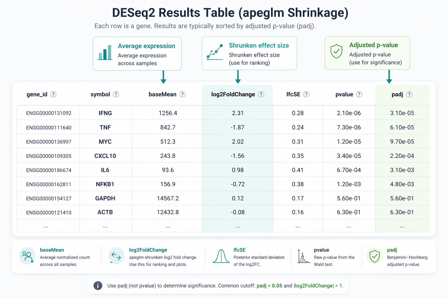
# Add gene symbol column to the resultsres_df <- as.data.frame(res_shrunk) |> tibble::rownames_to_column("gene_id") |> mutate( # Strip version number from Ensembl ID (e.g. ENSG00000123456.14 -> ENSG00000123456) gene_id_clean = sub("\\..*", "", gene_id), symbol = mapIds( org.Hs.eg.db, keys = gene_id_clean, column = "SYMBOL", keytype = "ENSEMBL", multiVals = "first" ) ) |> # Move symbol to the front select(gene_id, symbol, baseMean, log2FoldChange, lfcSE, pvalue, padj) |> arrange(padj, desc(abs(log2FoldChange)))
cat("Total genes in results:", nrow(res_df), "\n")Export DEG tables
# All genes, ranked by adjusted p-valuewrite_csv(res_df, "results/deseq2_all_genes.csv")
# Significant DEGs only: padj < 0.05 and |log2FC| > 1 (2-fold change)degs <- res_df |>  filter(padj < 0.05, abs(log2FoldChange) > 1)
write_csv(degs, "results/deseq2_significant_degs.csv")
cat("Significant DEGs (padj < 0.05, |LFC| > 1):", nrow(degs), "\n")cat("  Upregulated:  ", sum(degs$log2FoldChange > 0), "\n")cat("  Downregulated:", sum(degs$log2FoldChange < 0), "\n")
What the results columns mean
baseMean is the average normalized count across all samples. log2FoldChange is the shrunken effect size. lfcSE is the posterior standard deviation. pvalue is the raw Wald test p-value. padj is the Benjamini-Hochberg adjusted p-value. Always use padj for significance thresholds, never the raw pvalue.
A Complete Runnable Script
Here is the full analysis from import to export in one script. Save it as run_deseq2.R.
#!/usr/bin/env Rscript# Full DESeq2 analysis from Salmon quant.sf files to DEG table
suppressPackageStartupMessages({  library(tximeta)  library(DESeq2)  library(apeglm)  library(AnnotationDbi)  library(org.Hs.eg.db)  library(dplyr)  library(readr)})
# ── 1. Build sample table ────────────────────────────────────────────quant_dirs   <- list.dirs("results/quant", recursive = FALSE, full.names = TRUE)sample_names <- sub("_quant$", "", basename(quant_dirs))metadata     <- read_csv("sample_sheet.csv") |>                  arrange(match(sample_id, sample_names))
coldata <- data.frame(  names     = sample_names,  files     = file.path(quant_dirs, "quant.sf"),  condition = factor(metadata$condition),  row.names = sample_names)coldata$condition <- relevel(coldata$condition, ref = "control")stopifnot(all(file.exists(coldata$files)))
# ── 2. Import with tximeta ───────────────────────────────────────────se  <- tximeta(coldata)gse <- summarizeToGene(se)
# ── 3. Build DESeqDataSet ────────────────────────────────────────────dds  <- DESeqDataSet(gse, design = ~ condition)keep <- rowSums(counts(dds) >= 10) >= 3dds  <- dds[keep, ]cat("Genes after filtering:", nrow(dds), "\n")
# ── 4. Run DESeq2 ────────────────────────────────────────────────────dds <- DESeq(dds)
# ── 5. Extract results with apeglm shrinkage ─────────────────────────coef_name  <- grep("condition_", resultsNames(dds), value = TRUE)[1]res_shrunk <- lfcShrink(dds, coef = coef_name, type = "apeglm")
# ── 6. Annotate and export ───────────────────────────────────────────res_df <- as.data.frame(res_shrunk) |>  tibble::rownames_to_column("gene_id") |>  mutate(    gene_id_clean = sub("\\..*", "", gene_id),    symbol = mapIds(org.Hs.eg.db, keys = gene_id_clean,                    column = "SYMBOL", keytype = "ENSEMBL", multiVals = "first")  ) |>  select(gene_id, symbol, baseMean, log2FoldChange, lfcSE, pvalue, padj) |>  arrange(padj, desc(abs(log2FoldChange)))
dir.create("results/deseq2", showWarnings = FALSE)write_csv(res_df, "results/deseq2/all_genes.csv")write_csv(filter(res_df, padj < 0.05, abs(log2FoldChange) > 1),          "results/deseq2/significant_degs.csv")
cat("Analysis complete.\n")cat("Results written to results/deseq2/\n")
Run it from the terminal:
conda activate r-rnaseqRscript run_deseq2.RManual DESeq2 vs NotchBio: From quant.sf to DEG Table
The R workflow above is rigorous and reproducible. It still requires the r-rnaseq environment from the Ubuntu and macOS setup guide, a working AnnotationDbi installation, and careful attention to reference levels and design formula construction.
NotchBio runs the equivalent DESeq2 pipeline automatically when you upload Salmon outputs or complete the upstream quantification within the platform. The design formula, size factor estimation, dispersion plots, apeglm shrinkage, and annotated results table are all produced without writing a line of R.
| Step | Manual R Pipeline | NotchBio |
|---|---|---|
| Install DESeq2 + apeglm | BiocManager or conda, 5-10 min | Not required |
| Build sample table | Write coldata DataFrame manually | Auto-built from metadata |
| Set reference level | relevel() before DESeqDataSet | UI dropdown |
| Design formula | Typed manually, easy to get wrong | Guided form |
| Batch correction | Add batch to formula manually | Detected from metadata |
| Low-count filtering | rowSums() filter written by hand | Automatic |
| apeglm shrinkage | lfcShrink() with correct coef name | Always on |
| Gene symbol annotation | AnnotationDbi mapIds() | Included in results table |
| Export DEG table | write_csv() | Download from dashboard |
| Time to first results | 30-60 min including debugging | 10 min from quant.sf upload |
If you want publication-ready DEG tables from your Salmon outputs without managing an R environment, notchbio.app runs the same pipeline on our infrastructure.
Further reading
Read another related post
What Is a Count Matrix and Why Does It Matter
Raw counts, TPM, FPKM, and DESeq2-normalized values each represent expression differently. What each one is, why it matters, and which to use downstream.
Research GuideExperimental Design Mistakes in Differential Expression
Replicates, confounders, paired designs, and pseudoreplication: the experimental design decisions that decide whether your DESeq2 results hold up.
Research GuideWhy Your Choice of Reference Genome Changes Your Results
GENCODE, Ensembl, UCSC, and RefSeq annotate the same genome differently. How that choice changes RNA-seq alignment, quantification, and your DEG list.