Tutorial

How to Build a Counts Matrix from featureCounts and Salmon in Python

By Abdullah Shahid · April 22, 2026 · 11 min read

Every RNA-seq pipeline eventually reaches the same bottleneck: you have counts, but they are spread across twelve separate files with columns you do not need, gene IDs in a format your downstream tool does not accept, and fractional values that DESeq2 will refuse to model.

Building a clean count matrix is not glamorous work. But it is the step that most tutorials skip over, which is why so many DESeq2 runs fail with cryptic errors about non-integer inputs, mismatched sample names, or missing genes.

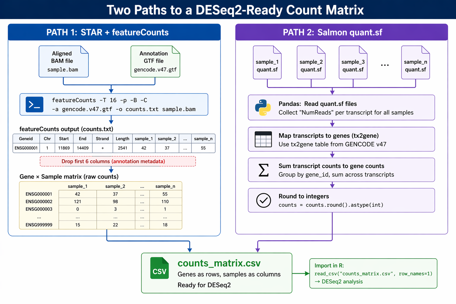
This tutorial covers both paths in Python. If you used STAR in Blog 5, you will load featureCounts output. If you used Salmon in Blog 4, you will aggregate the quant.sf files. Either way, the final output is an integer gene-by-sample count matrix saved as a CSV, ready for DESeq2 in R or PyDESeq2 in Python.

We use the rnaseq conda environment from Blog 1.

A clean technical diagram showing two parallel paths to a DESeq2-ready count matrix. The left path is labeled STAR plus featureCounts and shows a BAM file icon flowing into a featureCounts command box with the GTF file as a second input, producing a TSV file with six header columns to drop and then a clean gene by sample matrix. The right path is labeled Salmon quant.sf and shows multiple quant.sf file icons flowing into a pandas aggregation step with a tx2gene mapping step beneath it, then summing transcript counts to gene counts and rounding to integers. Both paths converge into a single green output box labeled counts_matrix.csv showing genes as rows and samples as columns, ready for DESeq2. — Figure 1: Two paths to the same output. featureCounts reads BAM files and outputs a single wide table. Salmon produces one quant.sf per sample that must be loaded, aggregated, and converted to gene-level counts. Both produce an identical integer count matrix format.

Path A: Loading featureCounts Output into a pandas DataFrame

featureCounts writes all samples into a single file. From the seventh column onward, the read count results for each sample are shown. Columns 1 through 6 contain gene identifier, chromosome, start, end, strand, and length information. You drop those first six columns and keep only the counts.

Run featureCounts on your BAM files

If you have not run featureCounts yet, this is the command. Run it from your project root after completing the STAR alignment in Blog 5.

conda activate rnaseq

GTF="references/gencode.v47.annotation.gtf"
OUTFILE="results/counts/featurecounts_output.txt"

mkdir -p results/counts

# Run featureCounts on all STAR BAM files
featureCounts \
    -p \
    -t exon \
    -g gene_id \
    -a "$GTF" \
    -o "$OUTFILE" \
    -T 8 \
    -s 2 \
    results/star/*Aligned.sortedByCoord.out.bam

echo "featureCounts complete: $OUTFILE"

The -p flag counts paired-end fragments instead of individual reads. -t exon summarizes at the exon level and aggregates to gene level. -s 2 specifies reverse-strand counting for standard Illumina TruSeq stranded libraries. Use -s 0 for unstranded libraries.

Set strandedness correctly or silently halve your counts

The -s parameter must match your library protocol. For unstranded libraries use -s 0. For TruSeq stranded libraries (dUTP method, most common) use -s 2. For first-strand protocols use -s 1. If you set this wrong, featureCounts will run without error but count reads from the wrong strand, typically losing around 50% of your reads. Check the .summary output file and confirm that “Assigned” exceeds 60%.

Load the featureCounts output in Python

import pandas as pd

# Load the featureCounts output file
# The first line is a comment with the command; skip it with comment="#"
fc_raw = pd.read_csv(
    "results/counts/featurecounts_output.txt",
    sep       = "\t",
    comment   = "#",    # skip the command-line header comment
    index_col = 0       # gene ID becomes the index
)

print(f"Raw featureCounts shape: {fc_raw.shape}")
# (58780, 17)  — 58780 genes, 6 annotation cols + 11 sample cols

print(fc_raw.columns.tolist()[:8])
# ['Chr', 'Start', 'End', 'Strand', 'Length',
#  'results/star/ctrl_1_Aligned.sortedByCoord.out.bam',
#  'results/star/ctrl_2_Aligned.sortedByCoord.out.bam', ...]

# Drop the annotation columns (Chr, Start, End, Strand, Length)
counts_fc = fc_raw.drop(columns=["Chr", "Start", "End", "Strand", "Length"])

# Clean up sample names: strip the full path and the BAM suffix
counts_fc.columns = (
    counts_fc.columns
    .str.replace(r"results/star/", "", regex=False)
    .str.replace(r"_Aligned\.sortedByCoord\.out\.bam", "", regex=True)
)

print(f"Cleaned counts shape: {counts_fc.shape}")
print(counts_fc.head(3))
#                     ctrl_1   ctrl_2  ctrl_3  treat_1  treat_2  treat_3
# ENSG00000000003.14      42      38       51       87       91       79
# ENSG00000000419.12     523     498      541      612      634      601
# ENSG00000000457.13     289     271      304      198      187      201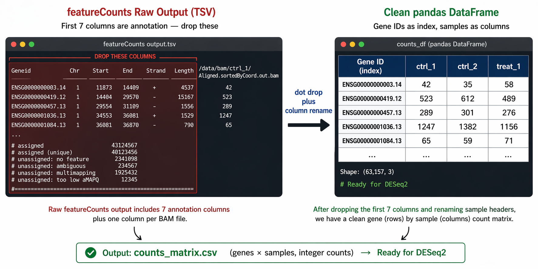

A side-by-side diagram of a terminal window showing featureCounts raw output on the left with the first seven columns labeled Geneid Chr Start End Strand Length and then a long BAM file path as the column header, with annotation columns highlighted in red as drop these; and on the right a clean pandas DataFrame showing only the gene ID as index and short sample names ctrl_1 ctrl_2 treat_1 as column headers with integer counts filling each cell. An arrow labeled dot drop plus column rename connects the two panels. — Figure 2: featureCounts output before and after cleanup. The raw file contains six annotation columns before the count columns, and sample column names are full BAM file paths. Two pandas operations handle both issues.

Path B: Aggregating Salmon quant.sf Files into a Count Matrix

Salmon produces one quant.sf file per sample. Each file has one row per transcript, not per gene. You need to load all files, aggregate from transcript to gene level using a tx2gene map, and round the estimated counts to integers.

Step 1: Load all quant.sf files

from pathlib import Path

# Find all quant.sf files
quant_dirs  = sorted(Path("results/quant").glob("*_quant"))
sample_names = [d.name.replace("_quant", "") for d in quant_dirs]

print(f"Found {len(sample_names)} samples: {sample_names[:4]}")

# Load each quant.sf and extract the NumReads column
parts = []
for sample, qdir in zip(sample_names, quant_dirs):
    qf = pd.read_csv(
        qdir / "quant.sf",
        sep       = "\t",
        index_col = "Name",
        usecols   = ["Name", "NumReads"]
    ).rename(columns={"NumReads": sample})
    parts.append(qf)

# Merge into a single transcript-level count matrix
tx_counts = pd.concat(parts, axis=1)

print(f"Transcript-level matrix: {tx_counts.shape}")
# (251638, 12)  for GENCODE v47 with 12 samples
print(tx_counts.head(3))

Step 2: Build a transcript-to-gene map from the GENCODE GTF

def build_tx2gene(gtf_path: str) -> pd.DataFrame:
    """
    Parse a GENCODE GTF and return a DataFrame mapping
    transcript_id to gene_id and gene_name.
    """
    rows = []
    with open(gtf_path) as fh:
        for line in fh:
            if line.startswith("#") or "\ttranscript\t" not in line:
                continue
            attrs = line.strip().split("\t")[8]

            # Parse key "value" pairs from the attribute field
            attr_dict = {}
            for item in attrs.split(";"):
                item = item.strip()
                if " " in item:
                    key, val = item.split(" ", 1)
                    attr_dict[key] = val.strip('"')

            tx   = attr_dict.get("transcript_id", "")
            gene = attr_dict.get("gene_id", "")
            name = attr_dict.get("gene_name", "")

            if tx and gene:
                rows.append({"transcript_id": tx,
                             "gene_id": gene,
                             "gene_name": name})

    return pd.DataFrame(rows).drop_duplicates(subset="transcript_id")


tx2gene = build_tx2gene("references/gencode.v47.annotation.gtf")
print(f"tx2gene rows: {len(tx2gene)}")
# 246,624 unique transcripts

print(tx2gene.head(3))
#          transcript_id          gene_id  gene_name
# ENST00000456328.2  ENSG00000223972.5  DDX11L2
# ENST00000450305.2  ENSG00000223972.5  DDX11L2
# ENST00000488147.1  ENSG00000227232.5  WASH7P

Cache the tx2gene table to avoid re-parsing the GTF every run

The GTF parse above takes 30 to 90 seconds for GENCODE v47. Save the result to a CSV and load it on subsequent runs: tx2gene.to_csv("references/tx2gene_v47.csv", index=False). Then replace the build_tx2gene() call with pd.read_csv("references/tx2gene_v47.csv").

Step 3: Aggregate transcript counts to gene level

# Salmon's GENCODE headers include pipe-separated fields: strip to transcript ID only
tx_counts.index = tx_counts.index.str.split("|").str[0]

# Map each transcript to its gene
tx2gene_dict = dict(zip(tx2gene["transcript_id"], tx2gene["gene_id"]))
tx_counts["gene_id"] = tx_counts.index.map(tx2gene_dict)

# Report unmapped transcripts
n_unmapped = tx_counts["gene_id"].isna().sum()
print(f"Unmapped transcripts: {n_unmapped} of {len(tx_counts)}")
# Unmapped transcripts: 423 of 251638  (novel/unannotated transcripts)

# Drop unmapped and sum to gene level
gene_counts_salmon = (
    tx_counts.dropna(subset=["gene_id"])
    .groupby("gene_id")
    .sum(numeric_only=True)
)

print(f"Gene-level Salmon counts: {gene_counts_salmon.shape}")
# (62703, 12)

Rounding, Validating, and Saving the Count Matrix

Salmon outputs fractional estimated counts, not integers. DESeq2 requires integer counts. Round with .round().astype(int).

This step applies to the Salmon path only. featureCounts already produces integers.

# Salmon path: round estimated counts to integers
counts_salmon = gene_counts_salmon.round().astype(int)

# Verify no negative values crept in (should never happen, but check)
assert (counts_salmon >= 0).all().all(), "Negative counts found"

# Check for all-zero genes (genes with no counts across any sample)
n_zero_genes = (counts_salmon.sum(axis=1) == 0).sum()
print(f"All-zero genes: {n_zero_genes}")

# Both paths: run these checks
def validate_count_matrix(counts: pd.DataFrame, source: str) -> None:
    """Quick sanity checks before saving."""
    print(f"\n=== Validating {source} counts ===")
    print(f"Shape:           {counts.shape}")
    print(f"Dtype:           {counts.dtypes.unique()}")
    print(f"Min value:       {counts.min().min()}")
    print(f"Max value:       {counts.max().max()}")
    print(f"NaN cells:       {counts.isna().sum().sum()}")
    print(f"All-zero genes:  {(counts.sum(axis=1) == 0).sum()}")
    print(f"Median depth:    {counts.sum(axis=0).median():.0f}")

validate_count_matrix(counts_fc,     "featureCounts")
validate_count_matrix(counts_salmon, "Salmon")

Save the count matrix

import os

os.makedirs("results/counts", exist_ok=True)

# featureCounts path
counts_fc.to_csv("results/counts/featurecounts_matrix.csv")

# Salmon path
counts_salmon.to_csv("results/counts/salmon_gene_matrix.csv")

print("Count matrices saved.")
print("  results/counts/featurecounts_matrix.csv")
print("  results/counts/salmon_gene_matrix.csv")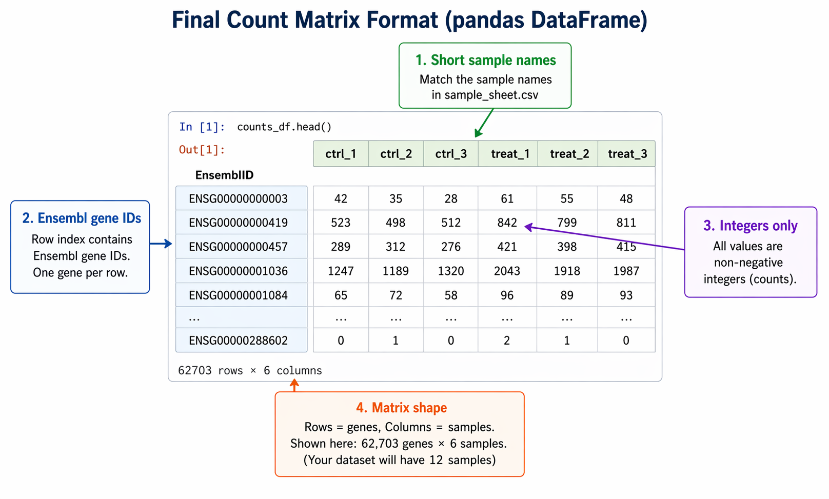

A clean annotated diagram of the final count matrix format showing a pandas DataFrame screenshot. The index column on the left contains Ensembl gene IDs like ENSG00000000003 and ENSG00000000419. The column headers across the top are sample names ctrl_1 ctrl_2 ctrl_3 treat_1 treat_2 treat_3. The body cells contain integer values between 0 and several thousand. Four callout boxes point to specific parts of the DataFrame: one to the index saying Ensembl gene IDs, one to the column headers saying short sample names matching sample_sheet.csv, one to a cell value saying integers only, and one to the bottom showing shape as 62703 rows by 12 columns. — Figure 3: The final count matrix format expected by DESeq2 and PyDESeq2. Ensembl gene IDs are the row index. Short sample names are column headers. Every cell is a non-negative integer. This is the input to DESeqDataSetFromMatrix() in R or DeseqDataSet() in Python.

Filtering Low-Count Genes Before DESeq2

You do not have to filter in Python. DESeq2 handles filtering internally. But removing genes that have essentially no expression across all samples speeds up computation and reduces the multiple testing burden.

A standard filter: keep genes with at least 10 counts in at least 3 samples.

def filter_low_counts(counts: pd.DataFrame,
                      min_count: int = 10,
                      min_samples: int = 3) -> pd.DataFrame:
    """
    Keep genes with at least min_count in at least min_samples samples.
    The min_samples value should match the size of your smallest group.
    """
    keep = (counts >= min_count).sum(axis=1) >= min_samples
    filtered = counts.loc[keep]
    print(f"Genes before filter: {len(counts)}")
    print(f"Genes after filter:  {len(filtered)}")
    return filtered

# Apply to either matrix before downstream analysis
counts_fc_filtered     = filter_low_counts(counts_fc)
counts_salmon_filtered = filter_low_counts(counts_salmon)

# Save filtered versions
counts_fc_filtered.to_csv("results/counts/featurecounts_filtered.csv")
counts_salmon_filtered.to_csv("results/counts/salmon_filtered.csv")

Aligning with Your Sample Sheet

The column order in your count matrix must match the row order of your sample metadata. A mismatch here is silent in DESeq2 but catastrophic for your results.

# Load sample metadata
metadata = pd.read_csv("sample_sheet.csv", index_col="sample_id")
print("Sample sheet order:")
print(metadata.index.tolist())

# Reorder count matrix columns to match the sample sheet
counts_final = counts_salmon_filtered.loc[:, metadata.index]

# Confirm alignment
assert list(counts_final.columns) == list(metadata.index), \
    "Sample order mismatch between count matrix and metadata"

print("Sample alignment verified.")
print(f"Final matrix: {counts_final.shape}")
# Final matrix: (19847, 12)

From here, the matrix is ready for DESeq2. In R, load it with read.csv() and pass it to DESeqDataSetFromMatrix(). In Python, load it with pd.read_csv() and transpose before passing to DeseqDataSet(). Both approaches are covered in Blog 7 and Blog 8.

Manual Count Matrix Assembly vs NotchBio

The steps above are genuinely tedious: featureCounts flag choices, GTF parsing, GENCODE header stripping, rounding, validation, and sample alignment. Getting any one of them wrong produces a count matrix that looks correct but gives you wrong differential expression results.

NotchBio assembles the count matrix automatically. Whether you quantified with Salmon or aligned with STAR, the platform converts the outputs into a validated integer matrix, checks sample alignment against your metadata, and passes it directly to the differential expression pipeline.

Step	Manual Python	NotchBio
Run featureCounts	`featureCounts -p -t exon -g gene_id -s 2`	Automatic after STAR alignment
Drop annotation columns	`drop(columns=["Chr","Start","End","Strand","Length"])`	Not required
Clean BAM path from column names	`str.replace()` regex	Not required
Load Salmon quant.sf files	Loop over 12 dirs, `pd.concat()`	Automatic
Parse GTF for tx2gene	Custom parser function, 30-90 sec	Pre-built for GENCODE v47, Ensembl
Strip GENCODE pipe headers	`str.split("	").str[0]`
Aggregate transcript to gene	`groupby("gene_id").sum()`	Automatic
Round estimated counts	`.round().astype(int)`	Automatic
Validate matrix	Manual assertion loop	Built-in, errors surface before DE runs
Align with sample sheet	`reindex(metadata.index)` with assertion	Auto-verified from upload metadata
Time to clean count matrix	30-60 min for 12 samples	2 min after quantification finishes

If you want to skip the pandas plumbing and go directly to differential expression, notchbio.app handles count matrix assembly as part of every analysis. Upload your Salmon outputs or STAR alignments, and the validated matrix is ready before you finish writing your methods section.

Read another related post

View all posts