ORA vs GSEA: A Side-by-Side Tutorial in R with clusterProfiler
After you have a DEG list, the next question is almost always: what biology does this represent? Over-representation analysis and gene set enrichment analysis are the two methods the field uses to answer that question, and they are not interchangeable. They ask different questions, require different inputs, and give results that are not directly comparable. Using the wrong one for your data, or using the right one incorrectly, is one of the most reliable ways to produce enrichment results that will not survive peer review.
This tutorial walks through both methods in clusterProfiler, the most widely used R package for functional enrichment analysis. It covers the conceptual distinction, the exact code for each method, the correct way to apply FDR correction, and how to read the results. Every code block runs on real DESeq2 output.
The Conceptual Difference
ORA (over-representation analysis) asks: given my list of significant genes, are any GO terms represented more often than expected by chance? It uses a one-sided Fisher exact test, comparing the fraction of your DEG list annotated to a term against the fraction of your background gene set annotated to the same term. It requires two inputs: a list of significant genes and a background gene set.
GSEA asks: is a GO term systematically enriched at the extremes of a ranked list of all my genes? It does not require a significance cutoff. Every tested gene participates, ordered from most upregulated to most downregulated by some continuous statistic, typically the DESeq2 Wald statistic. The enrichment score measures how much a gene set’s members cluster at the top or bottom of that ranking. GSEA was first described by Subramanian et al. in PNAS (2005) and has been one of the most cited methods in computational biology since.
The practical consequence of this difference is substantial. ORA with a strict fold change cutoff may miss a pathway where many genes show modest, consistent upregulation that does not individually cross your threshold. GSEA captures exactly that signal because it uses the full ranking. Conversely, ORA gives you a cleaner story when a small, specific set of genes is dramatically changed and the rest of the transcriptome is quiet.
ORA without a proper background gene set is statistically wrong
The background for ORA must be the set of genes that were actually tested in your differential expression analysis, not the full genome. If you use the full genome as background, you inflate the denominator of the Fisher test and make GO terms appear enriched when they are not. In clusterProfiler, pass the universe argument to enrichGO as the gene IDs of all genes with a non-NA adjusted p-value from DESeq2. Omitting the universe argument causes enrichGO to default to the full annotation database, which is incorrect for RNA-seq data.
Setup and Data Preparation
library(DESeq2)library(clusterProfiler)library(enrichplot)library(org.Hs.eg.db)library(ggplot2)
# Load DESeq2 results (shrunken, from lfcShrink)# Assumes you have already run DESeq2 and saved res_shrunkres_df <- as.data.frame(res_shrunk) |>  tibble::rownames_to_column("ensembl_id") |>  dplyr::filter(!is.na(padj))
# All tested genes: this is the correct ORA backgroundbackground_genes <- res_df$ensembl_id
# Significant DEGs: padj < 0.05 and |log2FC| >= 1sig_genes <- res_df |>  dplyr::filter(padj < 0.05, abs(log2FoldChange) >= 1) |>  dplyr::pull(ensembl_id)
cat("Background (tested) genes:", length(background_genes), "\n")cat("Significant DEGs:          ", length(sig_genes), "\n")
# Ranked gene list for GSEA: all tested genes sorted by Wald statistic# Use stat from the UNSHRUNKEN results object (res, not res_shrunk)# The Wald statistic is more appropriate than log2FC for rankingranked_genes <- res_df$statnames(ranked_genes) <- res_df$ensembl_idranked_genes <- sort(ranked_genes[!is.na(ranked_genes)], decreasing = TRUE)
cat("Genes in GSEA ranking:     ", length(ranked_genes), "\n")
Note the distinction between the objects: sig_genes is for ORA, background_genes is the ORA universe, and ranked_genes is for GSEA. These serve different roles and cannot be substituted for each other.
Running ORA with enrichGO
# Over-representation analysis on Biological Process GO termsora_result <- enrichGO(  gene          = sig_genes,  universe      = background_genes,   # correct background: all tested genes  OrgDb         = org.Hs.eg.db,  keyType       = "ENSEMBL",  ont           = "BP",               # Biological Process; also try "MF" and "CC"  pAdjustMethod = "BH",               # Benjamini-Hochberg FDR correction  pvalueCutoff  = 0.05,  qvalueCutoff  = 0.20,               # q-value is an additional FDR measure  readable      = TRUE                # converts gene IDs to gene symbols in output)
# How many terms were significant?cat("Significant ORA terms:", nrow(as.data.frame(ora_result)), "\n")
# Reduce redundant terms using semantic similarity# The simplify() function removes GO terms that are too similar to each otherora_simplified <- simplify(  ora_result,  cutoff    = 0.7,           # similarity threshold; lower = more aggressive pruning  by        = "p.adjust",  select_fun = min)
cat("Terms after simplify():", nrow(as.data.frame(ora_simplified)), "\n")
The simplify() function from the enrichplot package removes GO terms that share a high proportion of their annotated genes. Parent-child relationships in the GO hierarchy mean that “inflammatory response” and “regulation of inflammatory response” will often co-appear in ORA results. After simplify(), the list is shorter and more interpretable.
# Visualize ORA results as a dotplotdotplot(ora_simplified, showCategory = 20, title = "ORA: Biological Process (top 20, simplified)", font.size = 10) + ggplot2::theme(axis.text.y = element_text(size = 9))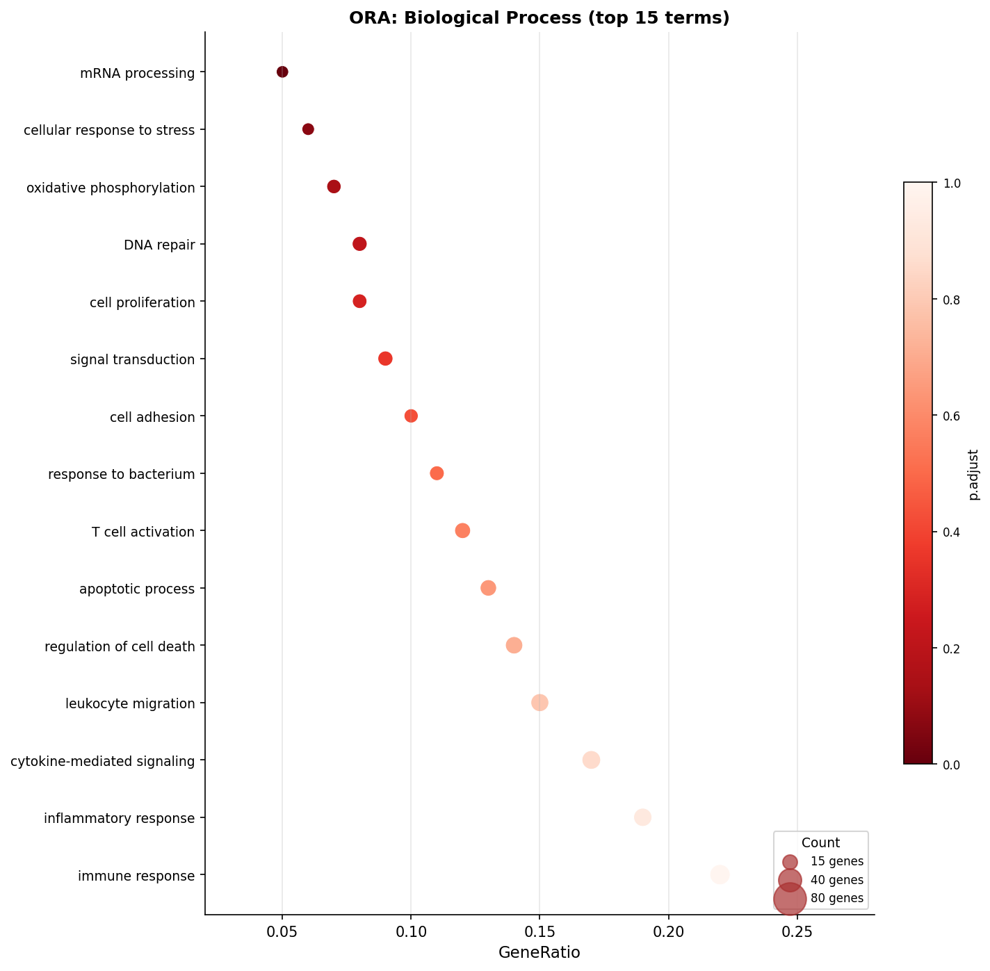
Running GSEA with gseGO
# Gene Set Enrichment Analysis on Biological Process GO terms# Input: all tested genes ranked by Wald statistic (continuous, no threshold)gsea_result <- gseGO(  geneList     = ranked_genes,        # named numeric vector, sorted descending  OrgDb        = org.Hs.eg.db,  keyType      = "ENSEMBL",  ont          = "BP",  minGSSize    = 10,                  # minimum gene set size to test  maxGSSize    = 500,                 # maximum gene set size to test  pvalueCutoff = 0.05,  pAdjustMethod = "BH",  verbose      = FALSE,  seed         = 42                   # set for reproducibility)
cat("Significant GSEA terms:", nrow(as.data.frame(gsea_result)), "\n")
# Simplify GSEA results the same way as ORAgsea_simplified <- simplify(gsea_result, cutoff = 0.7, by = "p.adjust", select_fun = min)
cat("Terms after simplify():", nrow(as.data.frame(gsea_simplified)), "\n")
Setting seed is important for reproducibility. The permutation procedure used to estimate significance in gseGO involves random sampling. Without a fixed seed, results will differ between runs, which complicates reproduction and version control.
The minGSSize and maxGSSize parameters control which gene sets are tested. Very small gene sets (fewer than 10 genes) produce unstable enrichment scores. Very large gene sets (more than 500 genes) often correspond to broad, non-specific terms like “metabolic process” that are rarely useful for biological interpretation. The defaults in gseGO are 10 and 500 respectively, which is appropriate for most RNA-seq experiments.
# Enrichment plot for the top GSEA term# This is the classic GSEA plot showing the running enrichment scoretop_term <- gsea_simplified@result$ID[1]gseaplot2(gsea_simplified, geneSetID = top_term, title = gsea_simplified@result$Description[1])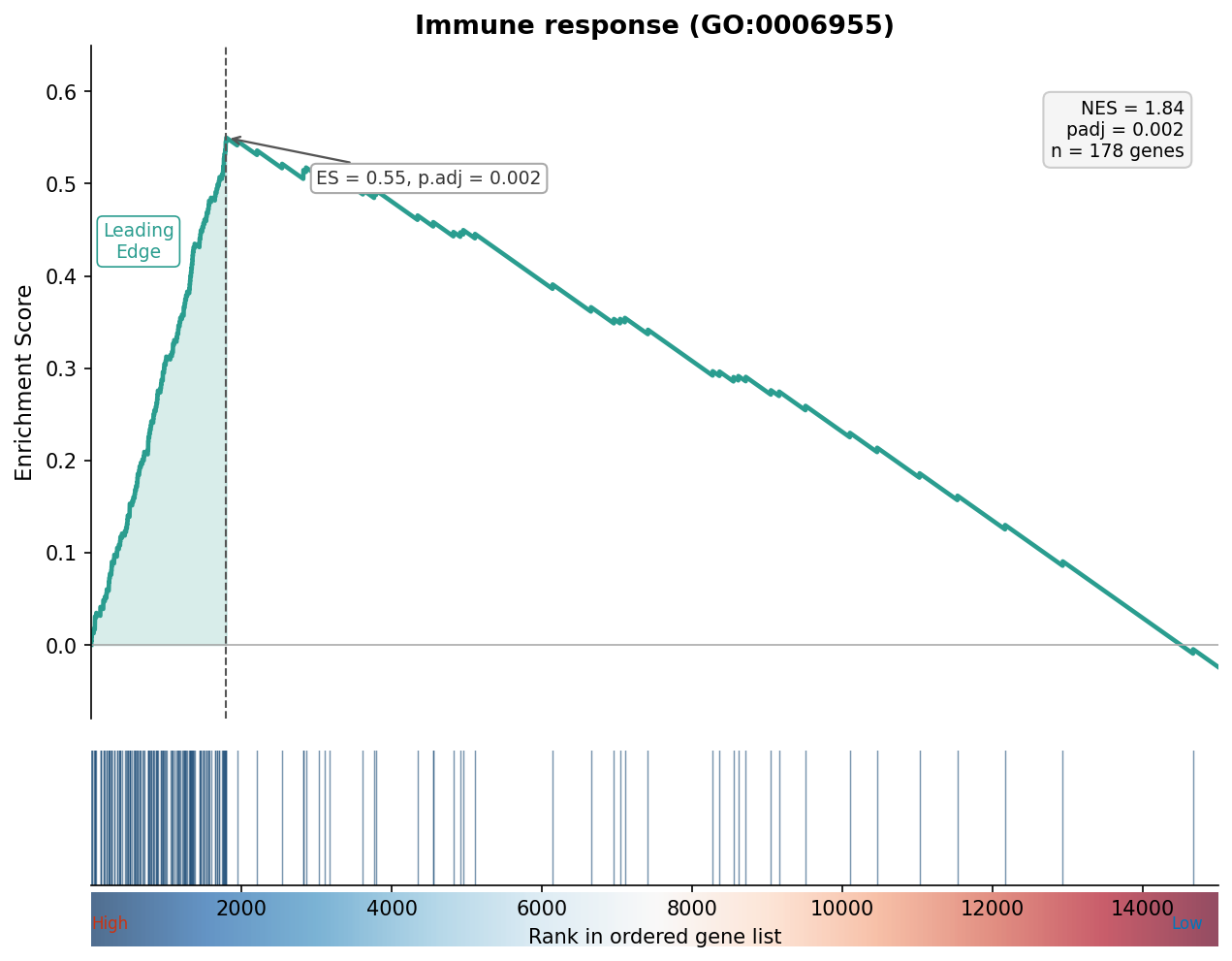
The Ridgeplot: Seeing Many Terms at Once
The ridgeplot is one of the most useful visualizations for GSEA because it shows the fold change distribution for all significant gene sets simultaneously. Each ridge represents one GO term, and the x-axis shows where the member genes fall in your fold change distribution.
# Ridgeplot: fold change distribution per significant gene setridgeplot(gsea_simplified, showCategory = 20, fill = "p.adjust") + ggplot2::labs( title = "GSEA ridgeplot: fold change distribution by GO term", x = "Log2 fold change" )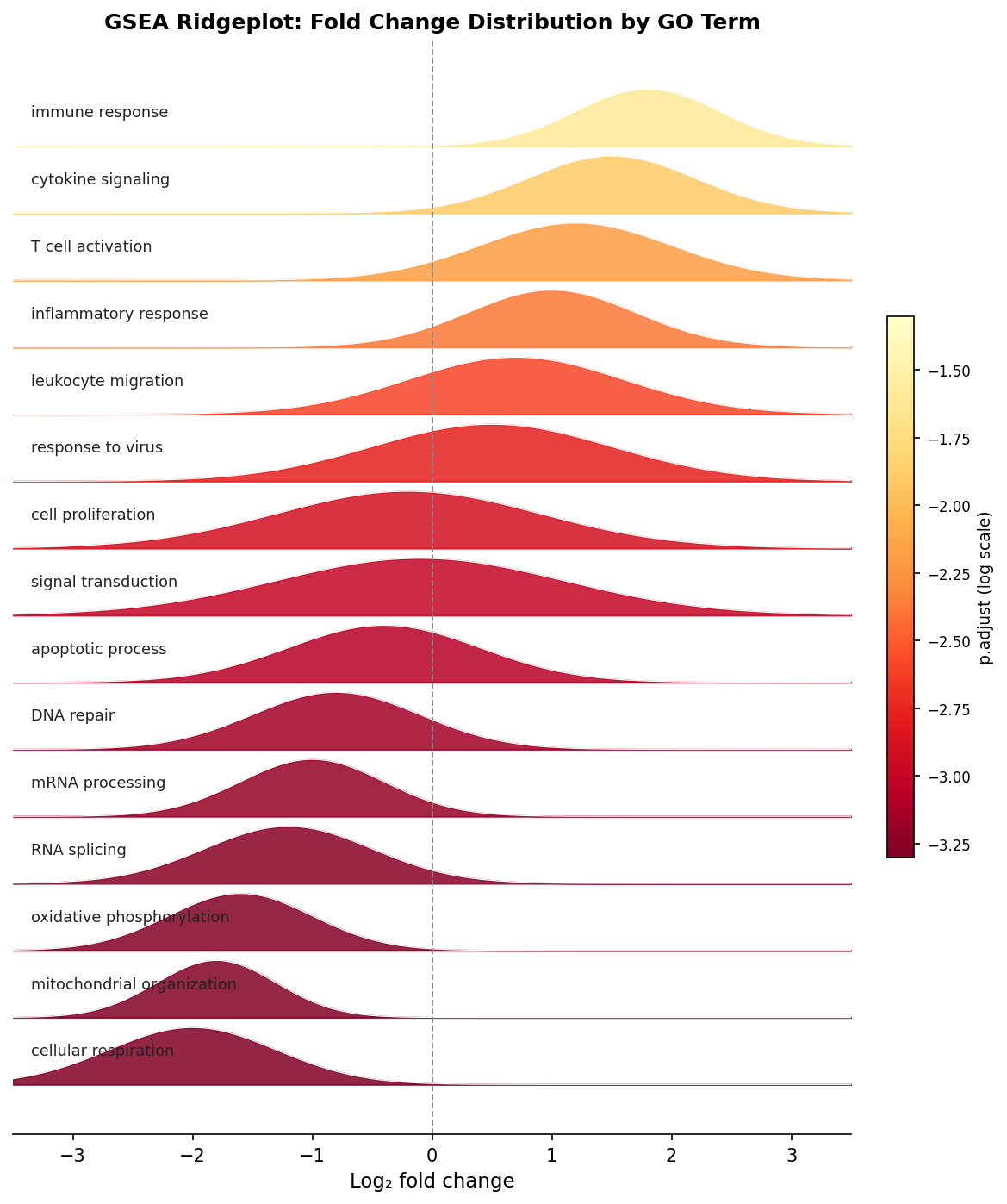
Interpreting and Comparing Results
ORA and GSEA will often identify overlapping terms, but they will not agree perfectly, and when they disagree the disagreement is informative.
A term that appears in ORA but not GSEA typically means a small, specific set of genes is strongly differentially expressed for that term, but the rest of the genome does not show a consistent signal in that direction. GSEA requires a genome-wide pattern; ORA only requires a local one.
A term that appears in GSEA but not ORA is the more interesting case. It usually means many genes are consistently but modestly shifted in one direction, without any individual gene crossing your fold change threshold. This is exactly the class of biology that ORA misses. Whole pathways under coordinated regulatory pressure, shifts in metabolic state, cell-type compositional changes reflected in the transcriptome: these often produce GSEA hits that never appear in ORA.
When a term appears in both, check that the direction is consistent. An ORA result cannot tell you direction (enrichment is enrichment), but GSEA tells you whether the enrichment is in the upregulated or downregulated tail via the sign of the normalized enrichment score (NES). Positive NES means enriched among upregulated genes; negative NES means enriched among downregulated genes.
When To Use Which
| Consideration | ORA | GSEA |
|---|---|---|
| Input required | DEG list and background | All tested genes, ranked by statistic |
| Threshold sensitivity | High: results change with padj and LFC cutoff | Low: uses the full continuous ranking |
| Background sensitivity | Very high: wrong background = wrong result | None: no hypergeometric test |
| Detects subtle coordinated shifts | No | Yes |
| Works with small DEG lists | Yes | Caution: ranking is noisy with few DEGs |
| Preferred for publication | Acceptable with correct background | Generally preferred by reviewers |
| Directionality in results | No (enrichment only) | Yes (positive or negative NES) |
| Computational cost | Low | Moderate (permutation-based) |
| clusterProfiler function | enrichGO() | gseGO() |
For most RNA-seq papers, running both and comparing them is more informative than choosing one. Report ORA results if you want a clean, specific gene-list-driven story. Report GSEA results if the biology involves coordinated pathway-level responses. If they agree, the result is stronger. If they disagree, understanding why is itself a biological finding.
The clusterProfiler documentation by the Yu lab is the authoritative reference for both methods and covers extensions to KEGG, Reactome, and custom gene sets. The original GSEA methodology paper by Subramanian et al. (2005) and the clusterProfiler 4.0 paper by Wu et al. are the primary citations for your methods section.
NotchBio runs both ORA and GSEA in parallel on every dataset, applies Benjamini-Hochberg correction by default, uses the tested gene universe as the ORA background, and runs simplify() on both result sets before returning the output. If you want publication-ready enrichment results without configuring each parameter manually, that is what the platform produces.
Related Reading
Further reading
Read another related post
Publication-Ready RNA-Seq Plots in ggplot2
Reviewer-ready RNA-seq plots in R: volcano with gene labels, z-score heatmap with annotation bars, PCA with variance explained, and journal export settings.
Research GuideThe One-Bioinformatician Problem: Stop Being The Bottleneck
If you are the only bioinformatician serving multiple PIs, you are the bottleneck. Here is how to scale with templates, self-service, and clear handoffs.
Research GuideWhy Your DESeq2 Log2 Fold Change Cutoff Of Zero Is Wrong
Filtering DEGs at log2FC greater than zero returns half your genome. How to choose a defensible cutoff, apply lfcShrink, and avoid the GO-term explosion.