Reducing GO Term Redundancy: simplify, rrvgo, and What Works
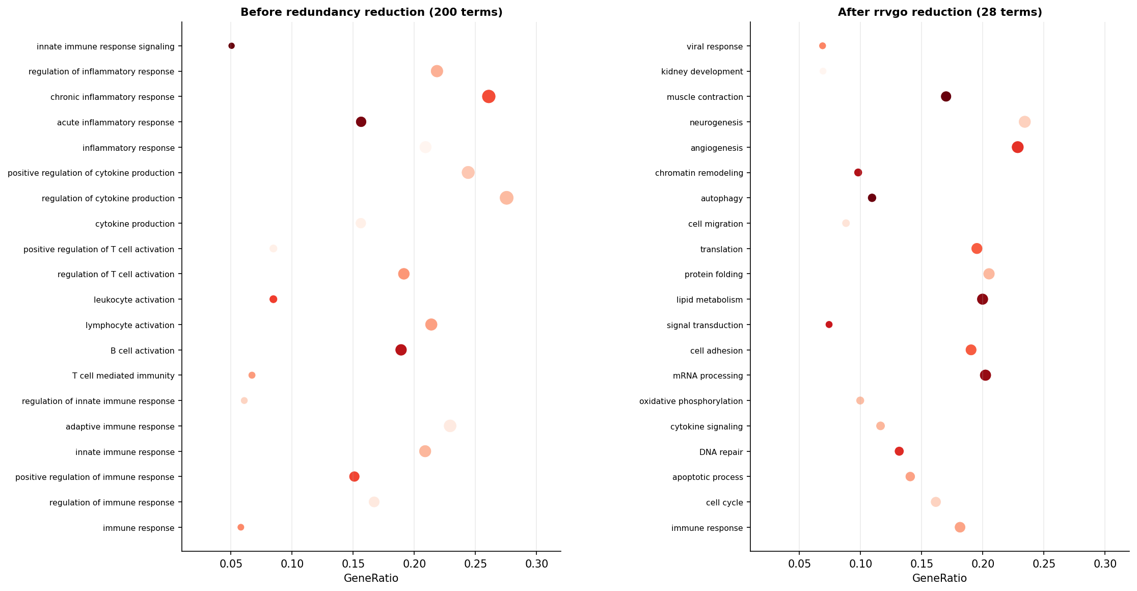
You ran ORA or GSEA, applied Benjamini-Hochberg correction, and got 300 significant GO terms. Now what? Presenting 300 terms in a paper is not an option. Manually curating them is not realistic. And simply picking the top 10 by adjusted p-value misses the fact that those 10 terms may all be near-identical siblings in the GO hierarchy, saying the same biological thing ten different ways.
The GO hierarchy is a directed acyclic graph. A parent term like “immune response” contains child terms like “innate immune response,” “adaptive immune response,” and dozens more specific children. When a gene set is enriched for any of those children, it is almost certainly enriched for the parent too. Standard enrichment analysis reports all of them. Your job is to collapse the redundant ones without losing the biological signal.
This tutorial covers three approaches in order of effort: simplify() from clusterProfiler, rrvgo from Bioconductor, and REVIGO as a web-based fallback. It also covers a custom uniqueness-score approach for the cases where all three run into problems.
Why Enrichment Outputs Hundreds of Similar Terms
The Gene Ontology is organized as a hierarchy where more specific terms inherit from broader ones. A gene annotated to “positive regulation of T cell proliferation” is also implicitly annotated to “regulation of T cell proliferation,” “T cell proliferation,” “lymphocyte proliferation,” “leukocyte proliferation,” “cell proliferation,” and so on up to “biological process.” When you run ORA or GSEA, all of these terms may test as significant if enough of your DEGs are annotated at any level.
This is not a bug in the enrichment software. It is a faithful reflection of the GO data structure. The redundancy is in the annotation, not the analysis. The result is that your 300 significant terms may represent only 20 to 30 distinct biological themes, each appearing in the output multiple times at different levels of specificity.
The goal of redundancy reduction is not to throw away information. It is to identify one representative term per cluster of semantically similar terms, so you can present the biological story in a form that is both accurate and readable.
Method 1: clusterProfiler simplify()
The fastest approach is simplify(), which ships with clusterProfiler and requires no additional installation. It works by computing pairwise semantic similarity between all significant terms using GOSemSim, then clustering the terms and selecting one representative per cluster.
library(clusterProfiler)library(enrichplot)library(org.Hs.eg.db)
# Assume ora_result is your enrichGO output from the previous tutorial# Apply simplify to remove redundant GO termsora_simplified <- simplify(  ora_result,  cutoff     = 0.7,          # similarity threshold; 0.5 is aggressive, 0.9 is lenient  by         = "p.adjust",   # pick the most significant term as representative  select_fun = min            # lower p.adjust = more significant)
# Compare before and aftercat("Terms before simplify():", nrow(as.data.frame(ora_result)), "\n")cat("Terms after simplify(): ", nrow(as.data.frame(ora_simplified)), "\n")
The cutoff parameter controls aggressiveness. A cutoff of 0.7 means two terms with semantic similarity above 0.7 will be merged into one cluster. Lower values (0.4 to 0.6) produce fewer, broader clusters. Higher values (0.8 to 0.9) produce more, tighter clusters with less reduction. For most RNA-seq papers, 0.7 is a reasonable default that reduces a 200-term list to roughly 30 to 60 representative terms.
simplify() works well for ORA results from enrichGO. It also works for GSEA results from gseGO. The key limitation is that it can only be applied to GO-based results from clusterProfiler. If you ran enrichment against KEGG, Reactome, or a custom gene set database, simplify() is not available.
Method 2: rrvgo
rrvgo is a dedicated Bioconductor package for GO term redundancy reduction by Sayols (2023). It is more flexible than simplify() because it accepts any list of GO term IDs and p-values as input, regardless of which enrichment tool produced them. It is heavily influenced by REVIGO and mimics its core algorithm in a programmatic interface.
rrvgo install issues and the most common fix
rrvgo depends on GOSemSim, which requires large annotation data packages that can fail to install on some systems due to memory or timeout constraints. If BiocManager::install(“rrvgo”) fails, try installing GOSemSim separately first: BiocManager::install(“GOSemSim”). Then install rrvgo. If the annotation database download fails mid-install, set options(timeout = 600) before trying again. On HPC systems with restricted internet access, you may need to pre-download the org.Hs.eg.db tarball and install locally using install.packages(“path/to/tarball”, repos = NULL, type = “source”).
# Install rrvgo if neededif (!requireNamespace("rrvgo", quietly = TRUE)) {  BiocManager::install("rrvgo")}
library(rrvgo)
# Extract GO term IDs and their scores from your ORA result# rrvgo needs GO IDs and a numeric score; use -log10(padj) so higher = more significantgo_terms  <- ora_result@result$IDgo_scores <- setNames(-log10(ora_result@result$p.adjust), go_terms)
# Step 1: Compute semantic similarity matrixsim_matrix <- calculateSimMatrix(  go_terms,  orgdb    = "org.Hs.eg.db",  ont      = "BP",           # must match the ontology you ran ORA/GSEA with  method   = "Rel"           # "Rel" (relevance) is a good default; also try "Wang")
# Step 2: Reduce based on similarity matrixreduced_terms <- reduceSimMatrix(  sim_matrix,  scores    = go_scores,     # higher scores = preferred as representative  threshold = 0.7,           # same logic as simplify(): 0.7 is a good default  orgdb     = "org.Hs.eg.db")
# How many clusters?cat("Clusters after rrvgo reduction:", length(unique(reduced_terms$cluster)), "\n")cat("Total input terms:             ", nrow(reduced_terms), "\n")
The reduced_terms object is a data frame with one row per input GO term. The cluster column identifies which representative term each input term was assigned to. The parentTerm column names the representative for that cluster.
# Visualize as a treemap# Each rectangle is one cluster; size proportional to number of terms in the clustertreemapPlot(reduced_terms)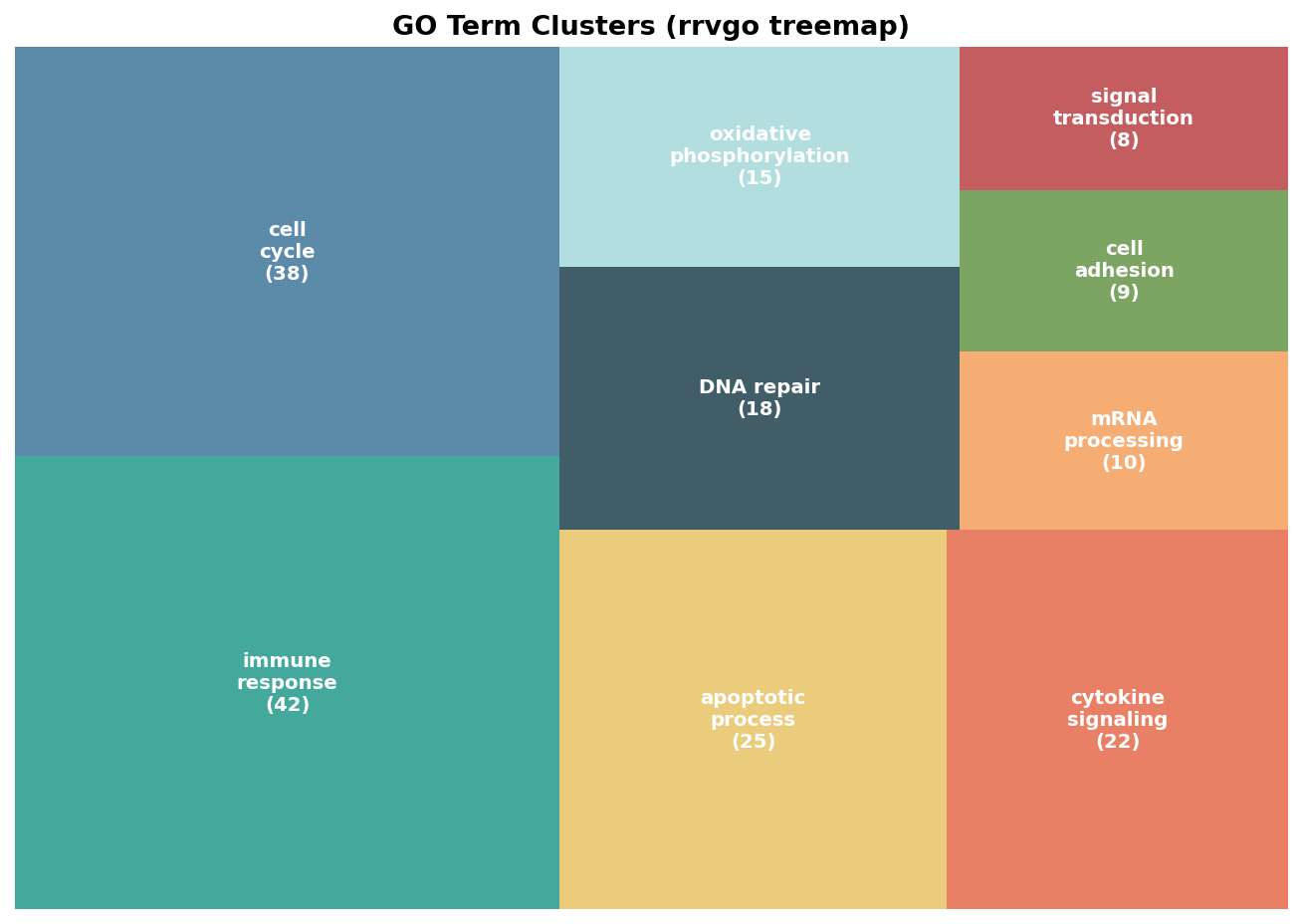
# Extract only the representative terms for reportingrepresentative_terms <- reduced_terms[reduced_terms$go == reduced_terms$parent, ]representative_terms <- representative_terms[order(representative_terms$score, decreasing = TRUE), ]
# Print the top 15 representative termshead(representative_terms[, c("go", "term", "score", "size")], 15)
The scatter plot is useful for exploring the semantic landscape. Each term is a point positioned by the first two components of a principal coordinates analysis of the similarity matrix. Terms near each other in the plot are semantically similar.
# Scatter plot: semantic similarity spacescatterPlot(sim_matrix, reduced_terms, algorithm = "pca", label.size = 3)Method 3: REVIGO Web Tool
REVIGO by Supek et al. (2011) is the original web-based tool for GO term redundancy reduction and remains useful as a quick fallback when rrvgo installation fails or when you need an interactive visualization to share with collaborators. The input is a list of GO term IDs and their p-values, pasted directly into the web interface.
The algorithm REVIGO uses is conceptually similar to rrvgo: it computes pairwise semantic similarity and selects representative terms. The main practical difference is that REVIGO runs online and does not require any local installation, but it is also limited to the GO annotation version it maintains internally, which may lag behind the Bioconductor annotation packages you used in your enrichment analysis.
To use REVIGO from R, export your GO term list first:
# Export GO terms and p-values for REVIGO inputrevigo_input <- data.frame(  go_id   = ora_result@result$ID,  padj    = ora_result@result$p.adjust)
write.table(revigo_input,            "revigo_input.txt",            sep       = "\t",            row.names = FALSE,            col.names = FALSE,            quote     = FALSE)
Paste the contents of revigo_input.txt into the REVIGO web interface at revigo.irb.hr. Select the appropriate organism and ontology. Download the results as a CSV and import back into R for any further processing or plotting.
Method 4: Custom Uniqueness Score Approach
When simplify() is unavailable (non-GO databases), rrvgo fails to install, and REVIGO does not match your annotation version, a custom approach based on term uniqueness is the last resort. This is also the approach to reach for when you want full control over which representative is chosen from each cluster.
The core idea is to compute a uniqueness score for each GO term, where uniqueness is defined as the fraction of that term’s annotated genes that do not appear in any other significant term. Terms with high uniqueness represent biology not captured by any other significant result and are the most information-dense candidates for reporting.
# Custom uniqueness-based filtering# Requires the gene sets for each significant GO termlibrary(dplyr)
# Extract the gene sets from the ORA resultgo_genesets <- ora_result@geneSets[ora_result@result$ID]
# Compute pairwise Jaccard similarity between gene setsjaccard_sim <- function(a, b) length(intersect(a, b)) / length(union(a, b))
compute_uniqueness <- function(go_id, all_genesets) {  term_genes  <- all_genesets[[go_id]]  other_genes <- unlist(all_genesets[names(all_genesets) != go_id])  unique_genes <- setdiff(term_genes, other_genes)  length(unique_genes) / length(term_genes)}
uniqueness_scores <- sapply(  names(go_genesets),  compute_uniqueness,  all_genesets = go_genesets)
# Filter: keep terms with uniqueness above 0.25# (at least 25% of their genes are not shared with any other significant term)unique_terms <- ora_result@result |>  dplyr::filter(ID %in% names(uniqueness_scores[uniqueness_scores > 0.25])) |>  dplyr::arrange(p.adjust)
cat("Terms after uniqueness filter:", nrow(unique_terms), "\n")
A uniqueness threshold of 0.25 is a reasonable starting point. Higher thresholds (0.4 to 0.5) produce a more stringent filter that keeps only the most distinct terms. Lower thresholds converge toward showing all terms. The right value depends on how correlated your significant terms are; examine the distribution of uniqueness scores first and choose a cutoff that separates the long tail of near-zero-uniqueness terms from the core of genuinely distinct ones.
Which Method To Use
| Method | Works for | Requires installation | Handles non-GO databases | Reproducible | Notes |
|---|---|---|---|---|---|
| simplify() | enrichGO, gseGO results only | No (ships with clusterProfiler) | No | Yes | Fastest; use first |
| rrvgo | Any GO term list with IDs | Yes (Bioconductor) | No | Yes | More flexible; good visualizations |
| REVIGO | Any GO term list | No (web tool) | No | Limited (web tool) | Good for sharing; annotation may lag |
| Custom uniqueness | Any enrichment result | No (base R + dplyr) | Yes | Yes | Last resort; full control |
The practical sequence is: try simplify() first for GO-based results, reach for rrvgo when you need more control or the scatter/treemap visualizations, use REVIGO when you want an interactive web-based workflow or when rrvgo installation fails, and fall back to the custom uniqueness approach when your enrichment results come from a non-GO database or when you want to control the representative-selection logic exactly.
NotchBio applies GO term redundancy reduction automatically on every enrichment analysis run, using simplify() with a default threshold of 0.7 for ORA results and rrvgo for the scatter plot visualization included in the run report. If you want to adjust the threshold or explore the full unreduced term list, both are available in the downloadable run outputs.
Related Reading
Further reading
Read another related post
How to Run DESeq2: From Count Matrix to Results
Step-by-step DESeq2 in R: build a DESeqDataSet, understand size factors and dispersion, run DESeq(), interpret the results columns, then shrink and filter DEGs.
TutorialSet Up a Bulk RNA-Seq Environment on Ubuntu and macOS
Install Miniforge, conda, bioconda, R 4.4, and DESeq2 for bulk RNA-seq: reproducible environments, version pinning, and fixes for common install errors.
TutorialHow to Quantify RNA-Seq Reads with Salmon
Step-by-step Salmon tutorial: build a decoy-aware index, run salmon quant on paired-end reads, read the quant.sf output, and import into DESeq2 with tximport.