Tutorial

How to Run Differential Expression in Python with PyDESeq2

By Abdullah Shahid · April 25, 2026 · 14 min read

rna-seq tutorial differential-expression bioinformatics

Most RNA-seq tutorials assume you are comfortable in R. If your lab runs everything in Python, the jump to R for a single DESeq2 step has always been an annoying cost.

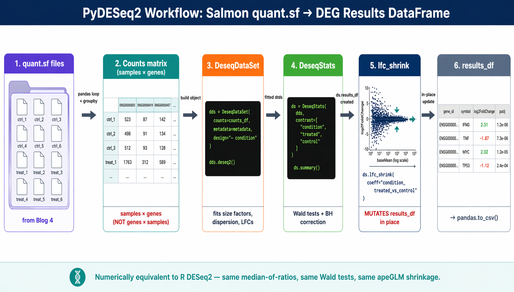
PyDESeq2 fixes that. It is a from-scratch Python implementation of the DESeq2 pipeline, maintained by the Owkin team, that produces results numerically equivalent to the R version. Same median-of-ratios normalization, same dispersion trend fitting, same Wald tests, same apeGLM shrinkage.

This tutorial walks through the full PyDESeq2 workflow. We load Salmon quant.sf files directly into a count matrix, build a DeseqDataSet, run the model, apply lfc_shrink(), and export a ranked DEG table. We continue from Blog 4 using your results/quant/ directory and the rnaseq conda environment from Blog 1.

Horizontal six-stage PyDESeq2 pipeline diagram showing Salmon quant.sf files flowing into a counts matrix with samples as rows and genes as columns, then into a DeseqDataSet object with metadata and design formula, then through deseq2() which runs size factors dispersion and GLM coefficients, then DeseqStats with a contrast list, then lfc_shrink with apeGLM, ending in a results_df DataFrame with columns baseMean log2FoldChange lfcSE pvalue padj — Figure 1: The complete PyDESeq2 workflow in Python. The key orientation difference from R is that PyDESeq2 expects the counts matrix as samples × genes, not genes × samples. Everything downstream is numerically equivalent to R DESeq2.

Why PyDESeq2 Exists and When to Use It

R DESeq2 is still the reference implementation. It has been cited over 60,000 times and is the most battle-tested differential expression tool in the field. If you already have an R pipeline that works, there is no reason to rewrite it in Python.

PyDESeq2 matters for three situations.

First, labs with a pure Python stack. If your upstream processing, visualization, and downstream analysis all happen in Python, PyDESeq2 removes the friction of switching languages for one step.

Second, integration with Python-native tools. PyDESeq2 plays well with scanpy, anndata, and the broader single-cell ecosystem. A DeseqDataSet is an AnnData subclass, so the same object can be passed to scanpy utilities.

Third, teams that want reproducibility without the R dependency burden. Bioconductor packages can be brittle to install, especially on Apple Silicon. A pure pip install pydeseq2 avoids that entire maintenance surface.

What PyDESeq2 does (and does not) replicate

PyDESeq2 implements the core DESeq2 pipeline: size factors, dispersion estimation, Wald tests, Cook’s filtering, independent filtering, apeGLM shrinkage, and multifactor designs. It does not currently implement the likelihood ratio test, rlog transformation, or some of the more niche R-side features. For the vast majority of two-group or multifactor differential expression analyses, it is a drop-in replacement.

How to Install PyDESeq2 in a Clean conda Environment

PyDESeq2 is a pip-only package. Install it into your rnaseq conda environment from Blog 1, or create a dedicated environment.

# Dedicated environment (recommended for first-time users)
conda create -n pydeseq2 python=3.11 -y
conda activate pydeseq2

# Install PyDESeq2 and the plotting stack
pip install pydeseq2==0.5.4
pip install pandas numpy matplotlib seaborn mygene

Verify the install:

import pydeseq2
print(pydeseq2.__version__)

How to Build a Count Matrix from Salmon quant.sf in Python

PyDESeq2 takes a raw counts matrix as input. You need to convert Salmon’s per-sample quant.sf files into a single DataFrame.

There are two paths. The simple one uses pandas directly. The more rigorous one uses pyroe or tximeta equivalents for proper transcript-to-gene aggregation. For a standard bulk RNA-seq analysis, the pandas path is sufficient.

The pandas-native approach

import pandas as pd
import numpy as np
from pathlib import Path

# List all quant directories
quant_dirs = sorted(Path("results/quant").glob("*_quant"))
sample_names = [d.name.replace("_quant", "") for d in quant_dirs]

# Load each quant.sf and extract NumReads column
counts_list = []
for sample, qdir in zip(sample_names, quant_dirs):
    qf = qdir / "quant.sf"
    df = pd.read_csv(qf, sep="\t")
    # Use transcript ID as index; take NumReads as the count column
    df = df.set_index("Name")[["NumReads"]].rename(columns={"NumReads": sample})
    counts_list.append(df)

# Merge all samples into one transcript-level matrix
transcript_counts = pd.concat(counts_list, axis=1)
print(f"Transcript-level counts shape: {transcript_counts.shape}")
# (251638, 12)   for GENCODE v47 with 12 samples

Aggregate to gene level using a tx2gene mapping

Salmon quantifies transcripts, not genes. DESeq2 models work at the gene level. Aggregate using a transcript-to-gene map built from the GENCODE GTF.

# Build tx2gene from the GENCODE GTF (downloaded in Blog 4)
def build_tx2gene_from_gtf(gtf_path: str) -> pd.DataFrame:
    """Extract transcript_id -> gene_id mapping from a GENCODE GTF."""
    rows = []
    with open(gtf_path) as fh:
        for line in fh:
            if line.startswith("#") or "\ttranscript\t" not in line:
                continue
            attrs = line.strip().split("\t")[8]
            attr_dict = dict(
                item.strip().split(" ", 1)
                for item in attrs.split(";")
                if item.strip()
            )
            tx = attr_dict.get("transcript_id", "").strip('"')
            gene = attr_dict.get("gene_id", "").strip('"')
            gene_name = attr_dict.get("gene_name", "").strip('"')
            if tx and gene:
                rows.append((tx, gene, gene_name))
    return pd.DataFrame(rows, columns=["transcript_id", "gene_id", "symbol"])

tx2gene = build_tx2gene_from_gtf("references/gencode.v47.annotation.gtf")
print(f"tx2gene mapping: {len(tx2gene)} transcripts")

# Note: Salmon uses the full GENCODE header as transcript ID (with pipes)
# Strip the pipe-delimited extras to match the tx2gene keys
transcript_counts.index = transcript_counts.index.str.split("|").str[0]

Now aggregate transcript counts to gene level. We sum counts across all transcripts of a gene.

# Map transcripts to genes
tx_to_gene_dict = dict(zip(tx2gene["transcript_id"], tx2gene["gene_id"]))
transcript_counts["gene_id"] = transcript_counts.index.map(tx_to_gene_dict)

# Drop transcripts that did not map (rare edge cases)
transcript_counts = transcript_counts.dropna(subset=["gene_id"])

# Sum to gene level
gene_counts = transcript_counts.groupby("gene_id").sum()

# Round estimated counts to integers (DESeq2 requires integer counts)
gene_counts = gene_counts.round().astype(int)

print(f"Gene-level counts shape: {gene_counts.shape}")
# Expected ~62,703 genes for GENCODE v47 human

PyDESeq2 expects samples as rows, not columns

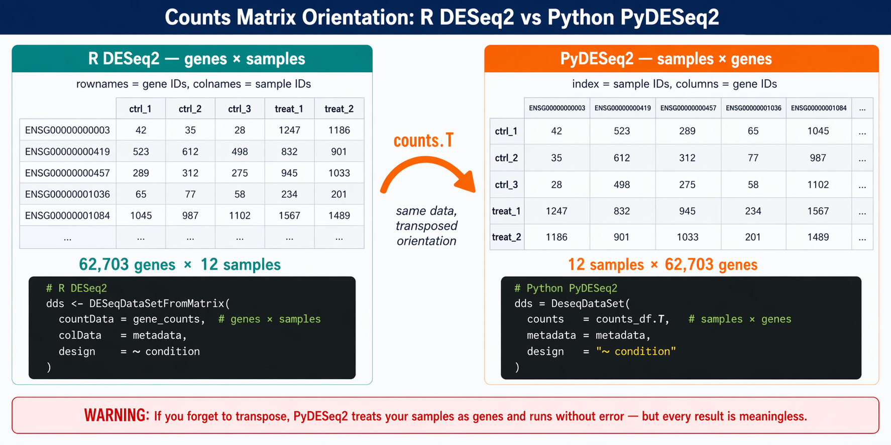
This is the biggest gotcha when moving from R to Python. R DESeq2 uses counts(dds) with genes as rows and samples as columns. PyDESeq2 reverses this. You must transpose your matrix so that rows are samples and columns are genes before passing it to DeseqDataSet.

Side-by-side comparison of counts matrix orientation: left panel labeled R DESeq2 shows a matrix with gene IDs on the rows and sample IDs on the columns, with dimension label 62703 genes × 12 samples; right panel labeled Python PyDESeq2 shows the transposed matrix with sample IDs on the rows and gene IDs on the columns, with dimension label 12 samples × 62703 genes; a big curved arrow labeled transpose connects the two panels; below both matrices is a code snippet showing counts.T to perform the transpose — Figure 2: The critical orientation difference between R DESeq2 and PyDESeq2. If you transpose incorrectly, PyDESeq2 will run without error but produce meaningless results because it will treat your samples as genes.

Transpose and align with metadata

# Transpose: samples × genes (PyDESeq2 convention)
counts_df = gene_counts.T
counts_df.index.name = "sample_id"

# Load sample metadata (from Blog 2)
metadata = pd.read_csv("sample_sheet.csv", index_col="sample_id")

# Ensure sample order matches between counts and metadata
counts_df = counts_df.loc[metadata.index]

# Sanity check
assert (counts_df.index == metadata.index).all(), "Sample order mismatch"
print(f"Counts: {counts_df.shape}  Metadata: {metadata.shape}")
# Counts: (12, 62703)  Metadata: (12, 3)

How to Build a DeseqDataSet and Run deseq2()

With the counts matrix correctly oriented, building a DeseqDataSet is straightforward.

from pydeseq2.dds import DeseqDataSet
from pydeseq2.default_inference import DefaultInference

# Filter out genes with very low counts (same logic as R)
# Keep genes with at least 10 counts in at least 3 samples
keep = (counts_df >= 10).sum(axis=0) >= 3
counts_filtered = counts_df.loc[:, keep]
print(f"Genes after filtering: {counts_filtered.shape[1]}")

# Configure inference (parallelism)
inference = DefaultInference(n_cpus=8)

# Build the DeseqDataSet
dds = DeseqDataSet(
    counts       = counts_filtered,
    metadata     = metadata,
    design       = "~ condition",     # formulaic syntax, same as R
    refit_cooks  = True,
    inference    = inference,
    quiet        = False
)

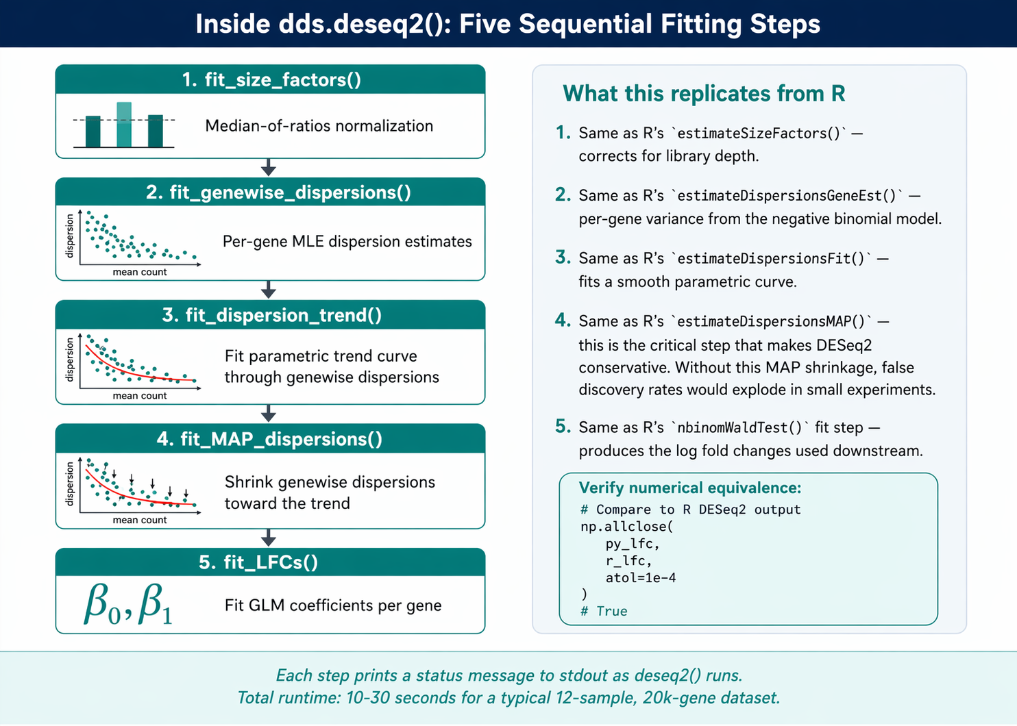
# Fit size factors, dispersion, and GLM coefficients
dds.deseq2()

The deseq2() method prints progress as it runs.

Fitting size factors...
... done in 0.2 seconds.

Fitting dispersions...
... done in 4.3 seconds.

Fitting dispersion trend curve...
... done in 0.1 seconds.

Fitting MAP dispersions...
... done in 4.1 seconds.

Fitting LFCs...
... done in 2.8 seconds.

Running Cook's outlier filtering...
... done in 0.3 seconds.

Each step corresponds exactly to the R DESeq2 pipeline. Size factor estimation uses median-of-ratios. Dispersion uses the same parametric trend fit with MAP shrinkage.

Vertical flowchart showing the five steps executed inside dds.deseq2(): step 1 fit_size_factors with median-of-ratios normalization icon, step 2 fit_genewise_dispersions with a dispersion vs mean scatter icon, step 3 fit_dispersion_trend_curve with a curve fitting icon, step 4 fit_MAP_dispersions with a shrinkage arrow pointing toward the curve, step 5 fit_LFCs with beta coefficients icon; each step is a rounded box with teal color and arrows connecting them top to bottom; right side shows a small callout noting that these are the same steps as R DESeq(), printed to stdout as deseq2() runs — Figure 3: What happens inside dds.deseq2(). These five steps are numerically equivalent to the internal steps of R's DESeq() function. The MAP dispersion fitting is the step that makes DESeq2 conservative and controls false discovery in small sample experiments.

Multifactor designs

If MultiQC from Blog 3 or the PCA from a previous analysis showed a batch effect, add batch to the design. The formulaic syntax matches R.

# Multifactor design: control for batch, test condition
dds_multi = DeseqDataSet(
    counts   = counts_filtered,
    metadata = metadata,
    design   = "~ batch + condition",    # batch is the covariate
    inference = inference,
)
dds_multi.deseq2()

The last term in the formula is the tested variable. ~ batch + condition tests the condition effect after adjusting for batch.

How to Run Wald Tests with DeseqStats

The DeseqStats class runs the actual differential expression test. It takes a fitted DeseqDataSet and a contrast specification.

from pydeseq2.ds import DeseqStats

# Contrast format: [variable, tested_level, reference_level]
# This computes LFC of treated vs control
ds = DeseqStats(
    dds,
    contrast = ["condition", "treated", "control"],
    alpha    = 0.05,
    inference = inference,
)

# Run the full statistical analysis
ds.summary()

The summary() method prints summary statistics and populates ds.results_df with the per-gene results.

Running Wald tests...
... done in 1.8 seconds.

Log2 fold change & Wald test p-value: condition treated vs control
                   baseMean  log2FoldChange     lfcSE       stat        pvalue           padj
ENSG00000000003      42.31        0.108164  0.172823   0.625870  5.314148e-01  7.618301e-01
ENSG00000000419     523.89        0.043257  0.096132   0.449980  6.527483e-01  8.340195e-01
ENSG00000000457     289.74       -0.194851  0.152904  -1.274326  2.025813e-01  4.372941e-01
...

out of 19,847 with nonzero total read count
adjusted p-value < 0.05
LFC > 0 (up)     : 1,203, 6.1%
LFC < 0 (down)   : 954, 4.8%
outliers         : 18, 0.1%
low counts       : 2,087, 10.5%

Access the results as a pandas DataFrame.

results = ds.results_df
print(results.head())
print(results.columns.tolist())
# ['baseMean', 'log2FoldChange', 'lfcSE', 'stat', 'pvalue', 'padj']

Contrast direction matters

The contrast ["condition", "treated", "control"] means LFC of treated vs control. Positive LFC = upregulated in treated. If you swap the order to ["condition", "control", "treated"], you get the same genes with flipped signs. Always document which direction is “up” in your results.

How to Apply apeGLM LFC Shrinkage

Raw maximum likelihood fold changes from DESeq2 are noisy for low-count genes. lfc_shrink() with apeGLM pulls these unreliable estimates toward zero while preserving well-supported large fold changes.

# Apply apeGLM shrinkage IN-PLACE on the ds object
ds.lfc_shrink(coeff="condition_treated_vs_control")

# Confirm the LFCs were shrunk
print(f"LFCs shrunk: {ds.shrunk_LFCs}")
# True

# The results_df is now updated with shrunken LFCs
results_shrunk = ds.results_df

lfc_shrink() mutates results_df in place

Unlike R’s lfcShrink() which returns a new object, PyDESeq2’s lfc_shrink() overwrites ds.results_df with the shrunken values. If you want to compare before and after shrinkage, save the raw results first. Once shrunk, there is no way to recover the original fold changes without re-running the Wald tests.

The right pattern is to save a copy before shrinking.

# Save raw LFCs first
results_raw = ds.results_df.copy()

# Then shrink
ds.lfc_shrink(coeff="condition_treated_vs_control")
results_shrunk = ds.results_df.copy()

# Now you can compare
print("Raw LFC range:   ", results_raw["log2FoldChange"].min(), results_raw["log2FoldChange"].max())
print("Shrunk LFC range:", results_shrunk["log2FoldChange"].min(), results_shrunk["log2FoldChange"].max())

The coefficient name to pass to lfc_shrink

The coeff argument must match a column name in the internal LFC matrix. PyDESeq2 formats these as {variable}_{level}_vs_{reference}.

# List the available coefficients
print(dds.LFC.columns.tolist())
# ['Intercept', 'condition_treated_vs_control']

For a simple two-group design, there will be one non-intercept coefficient. For multifactor designs, you will see multiple and need to pick the one matching your contrast.

How to Filter and Export Results with pandas

With results_shrunk in hand, filtering and exporting is standard pandas.

# Annotate with gene symbols using mygene
import mygene

mg = mygene.MyGeneInfo()

# Strip version numbers from Ensembl IDs
results_shrunk["gene_id_clean"] = results_shrunk.index.str.split(".").str[0]

# Query in batch (1000 genes at a time for speed)
gene_info = mg.querymany(
    results_shrunk["gene_id_clean"].tolist(),
    scopes  = "ensembl.gene",
    fields  = "symbol",
    species = "human",
    as_dataframe = True
)
symbol_map = gene_info["symbol"].to_dict()
results_shrunk["symbol"] = results_shrunk["gene_id_clean"].map(symbol_map)

# Reorder columns
results_shrunk = results_shrunk[[
    "symbol", "baseMean", "log2FoldChange", "lfcSE", "stat", "pvalue", "padj"
]]

# Sort by padj, tiebreaker by absolute LFC
results_shrunk = results_shrunk.sort_values(
    ["padj", "log2FoldChange"],
    ascending=[True, False],
    key=lambda c: c.abs() if c.name == "log2FoldChange" else c
)

Export full and filtered tables

from pathlib import Path
Path("results/pydeseq2").mkdir(parents=True, exist_ok=True)

# Full results
results_shrunk.to_csv("results/pydeseq2/all_genes.csv")

# Significant DEGs: padj < 0.05 and |LFC| > 1
degs = results_shrunk.query("padj < 0.05 and abs(log2FoldChange) > 1")
degs.to_csv("results/pydeseq2/significant_degs.csv")

print(f"Total genes tested:    {len(results_shrunk)}")
print(f"Significant DEGs:      {len(degs)}")
print(f"  Upregulated:         {(degs['log2FoldChange'] > 0).sum()}")
print(f"  Downregulated:       {(degs['log2FoldChange'] < 0).sum()}")

A Complete Runnable Script

Save this as run_pydeseq2.py and run it end to end.

#!/usr/bin/env python3
"""
run_pydeseq2.py: Full PyDESeq2 pipeline from Salmon quant.sf to DEG table.
"""
import pandas as pd
from pathlib import Path
from pydeseq2.dds import DeseqDataSet
from pydeseq2.ds  import DeseqStats
from pydeseq2.default_inference import DefaultInference

# ── 1. Load counts from Salmon ───────────────────────────────────────
quant_dirs = sorted(Path("results/quant").glob("*_quant"))
samples    = [d.name.replace("_quant", "") for d in quant_dirs]

parts = []
for s, q in zip(samples, quant_dirs):
    df = pd.read_csv(q / "quant.sf", sep="\t")
    df.index = df["Name"].str.split("|").str[0]
    parts.append(df[["NumReads"]].rename(columns={"NumReads": s}))
tx_counts = pd.concat(parts, axis=1)

# ── 2. Aggregate to gene level ───────────────────────────────────────
tx2gene = pd.read_csv("references/tx2gene.csv")       # precomputed
tx_counts["gene_id"] = tx_counts.index.map(
    dict(zip(tx2gene.transcript_id, tx2gene.gene_id))
)
gene_counts = (
    tx_counts.dropna(subset=["gene_id"])
             .groupby("gene_id").sum()
             .round().astype(int)
)

# ── 3. Transpose + metadata ──────────────────────────────────────────
counts_df = gene_counts.T
metadata  = pd.read_csv("sample_sheet.csv", index_col="sample_id")
counts_df = counts_df.loc[metadata.index]

# Filter low-count genes
keep = (counts_df >= 10).sum(axis=0) >= 3
counts_df = counts_df.loc[:, keep]

# ── 4. Fit DeseqDataSet ──────────────────────────────────────────────
inference = DefaultInference(n_cpus=8)
dds = DeseqDataSet(
    counts=counts_df, metadata=metadata,
    design="~ condition", inference=inference, quiet=False
)
dds.deseq2()

# ── 5. Wald test + shrinkage ─────────────────────────────────────────
ds = DeseqStats(dds, contrast=["condition", "treated", "control"],
                inference=inference)
ds.summary()
ds.lfc_shrink(coeff="condition_treated_vs_control")

# ── 6. Export ────────────────────────────────────────────────────────
out = Path("results/pydeseq2"); out.mkdir(parents=True, exist_ok=True)
ds.results_df.to_csv(out / "all_genes.csv")
ds.results_df.query("padj < 0.05 and abs(log2FoldChange) > 1") \
             .to_csv(out / "significant_degs.csv")

print("Done. Results in results/pydeseq2/")

Run it:

conda activate pydeseq2
python run_pydeseq2.py

Manual PyDESeq2 vs NotchBio

The PyDESeq2 pipeline above is clean and fully reproducible in Python. It still requires managing a conda environment, writing the count matrix aggregation code, and handling the samples × genes orientation correctly.

NotchBio runs the equivalent analysis automatically. Upload your Salmon outputs or let the platform run Salmon for you, then select the comparison you want. The counts matrix construction, model fitting, shrinkage, and annotation all happen server-side.

Step	Manual PyDESeq2	NotchBio
Install PyDESeq2	`pip install pydeseq2` in clean env	Not required
Build counts matrix	Loop over quant.sf, concat, aggregate to gene	Automatic
Transpose to samples × genes	`gene_counts.T` (critical gotcha)	Not applicable
Build tx2gene mapping	Parse GENCODE GTF	Pre-loaded for GENCODE, Ensembl
Set reference level	Order contrast list: [var, test, ref]	Dropdown in UI
Multifactor design	`design="~ batch + condition"`	Checkbox per variable
Run deseq2() + Wald	Two method calls, multiprocessing setup	Automatic
apeGLM shrinkage	`lfc_shrink()` with coeff name	Always on
Symbol annotation	`mygene` query in batches	Included in output
Export DEG tables	pandas to_csv	Download from dashboard
Time to first results	30-60 min including debugging	10 min from quant.sf upload

If you want to skip the counts matrix plumbing and environment management, notchbio.app runs PyDESeq2 and R DESeq2 interchangeably, with the same interface and the same annotated results table for either.

Read another related post

View all posts