DESeq2 Contrasts: Multiple Conditions and Multi-Factor Designs
The DESeq2 tutorial for a simple two-condition experiment fits on one page. The design formula is ~ condition, the contrast is c("condition", "treated", "control"), and resultsNames(dds) shows exactly one coefficient to interpret. Most real experiments are not this simple.
Three conditions with pairwise comparisons. A paired design where the same subjects appear in both conditions. A two-factor experiment where genotype and treatment interact. A time course where you want genes that change across timepoints rather than at any single one. Each of these requires a different design formula, a different contrast specification, and awareness of different failure modes.
This tutorial covers all four, with working code for each. The DESeq2 vignette at Bioconductor is the authoritative reference and should be consulted alongside this post for design-specific edge cases.
Setup: Reading the Design Matrix Before You Run
Before fitting any model, inspect the design matrix DESeq2 will build from your formula. This takes 30 seconds and catches most design mistakes before they propagate through the analysis.
library(DESeq2)
# Build the dds object with your chosen design formuladds <- DESeqDataSetFromMatrix(  countData = counts_matrix,  colData   = metadata,  design    = ~ condition          # placeholder; change for your design)
# Inspect the model matrix BEFORE running DESeq()# This shows exactly what each coefficient representsmodel.matrix(design(dds), colData(dds))
If the design matrix has a column of all zeros or two identical columns, the model is not full rank and DESeq() will fail with a rank error. Common causes: a factor with only one level, a covariate that is perfectly correlated with another factor, or including subject ID in a design where every subject appears in only one condition. Fix the design before proceeding.
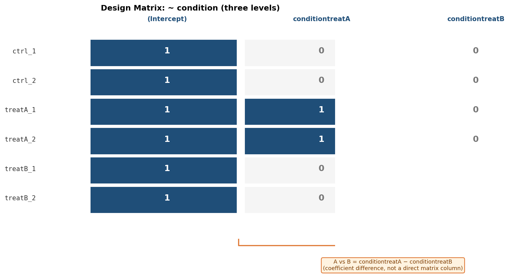
Case 1: Three or More Conditions, Pairwise Contrasts
The most common extension of the basic two-condition design is three conditions: a control plus two treatments, or three disease states, or three timepoints treated as categories.
# Metadata has a 'condition' column with three levels: "control", "treatA", "treatB"metadata$condition <- factor(metadata$condition,                              levels = c("control", "treatA", "treatB"))
dds <- DESeqDataSetFromMatrix(  countData = counts_matrix,  colData   = metadata,  design    = ~ condition)
dds <- DESeq(dds)
# Check what coefficients DESeq2 fittedresultsNames(dds)# Returns: "Intercept", "condition_treatA_vs_control", "condition_treatB_vs_control"
DESeq2 fits the reference level (control) as the intercept and each non-reference level as a coefficient relative to the reference. The resultsNames() output tells you exactly which comparisons are directly available.
# Direct comparisons against the reference levelres_A_vs_ctrl <- results(dds, name = "condition_treatA_vs_control")res_B_vs_ctrl <- results(dds, name = "condition_treatB_vs_control")
# The comparison NOT directly in resultsNames: A vs B# Use the contrast argument with the factor, numerator, denominatorres_A_vs_B <- results(dds,                       contrast = c("condition", "treatA", "treatB"))
The A vs B comparison is the one beginners most often miss. DESeq2 does not automatically output every pairwise comparison; it outputs comparisons against the reference level. For any non-reference-vs-non-reference comparison, use the contrast = c("factor", "numerator", "denominator") syntax.
Case 2: Paired Design with Subject as a Covariate
A paired design arises when the same biological subjects are measured under two or more conditions: patient samples before and after treatment, matched tumor and adjacent normal tissue, crossover experiments. The subject ID must be included in the design formula as a covariate to account for between-subject variability.
# Metadata columns: subject (e.g., "patient01"..."patient06"), condition ("before", "after")metadata$subject   <- factor(metadata$subject)metadata$condition <- factor(metadata$condition, levels = c("before", "after"))
dds <- DESeqDataSetFromMatrix(  countData = counts_matrix,  colData   = metadata,  design    = ~ subject + condition   # subject FIRST, condition LAST)
dds <- DESeq(dds)
# Extract the treatment effect, adjusted for subject differencesres_paired <- results(dds, name = "condition_after_vs_before")
The critical rule: the factor of interest must be the last term in the formula. Subject must come before condition. If you reverse the order, DESeq2 will model the subject effect as the quantity of interest and give you a nonsensical result.
The subject-as-covariate approach works when every subject appears in every condition, which is the standard paired design. It does not work when subjects are nested within one condition (each subject appears in only one group), which is a between-subject design that does not require pairing. For nested subjects, see the DESeq2 vignette section on group-specific condition effects.
Case 3: Two-Factor Design and Interaction Terms
A two-factor design has two independent variables: for example, condition (treated vs control) and genotype (wild-type vs mutant). The simplest two-factor formula models each factor as an additive main effect:
# Additive model: assumes the condition effect is the same across genotypes# and the genotype effect is the same across conditionsdds_additive <- DESeqDataSetFromMatrix( countData = counts_matrix, colData = metadata, design = ~ genotype + condition # condition last = factor of interest)dds_additive <- DESeq(dds_additive)resultsNames(dds_additive)# "Intercept", "genotype_mutant_vs_WT", "condition_treated_vs_control"The additive model gives you the average treatment effect across both genotypes and the average genotype effect across both conditions. Use it when you believe the two factors act independently.
When you want to ask “does the treatment effect differ between genotypes?”, add an interaction term:
# Interaction model: tests whether condition effect differs by genotypedds_interact <- DESeqDataSetFromMatrix( countData = counts_matrix, colData = metadata, design = ~ genotype + condition + genotype:condition)dds_interact <- DESeq(dds_interact)resultsNames(dds_interact)# "Intercept", "genotype_mutant_vs_WT",# "condition_treated_vs_control",# "genotypemutant.conditiontreated" <- this is the interaction term
# Is the treatment effect different in mutants vs WT?res_interaction <- results(dds_interact, name = "genotypemutant.conditiontreated")
# What is the treatment effect specifically in WT (the reference genotype)?res_treat_in_WT <- results(dds_interact, name = "condition_treated_vs_control")
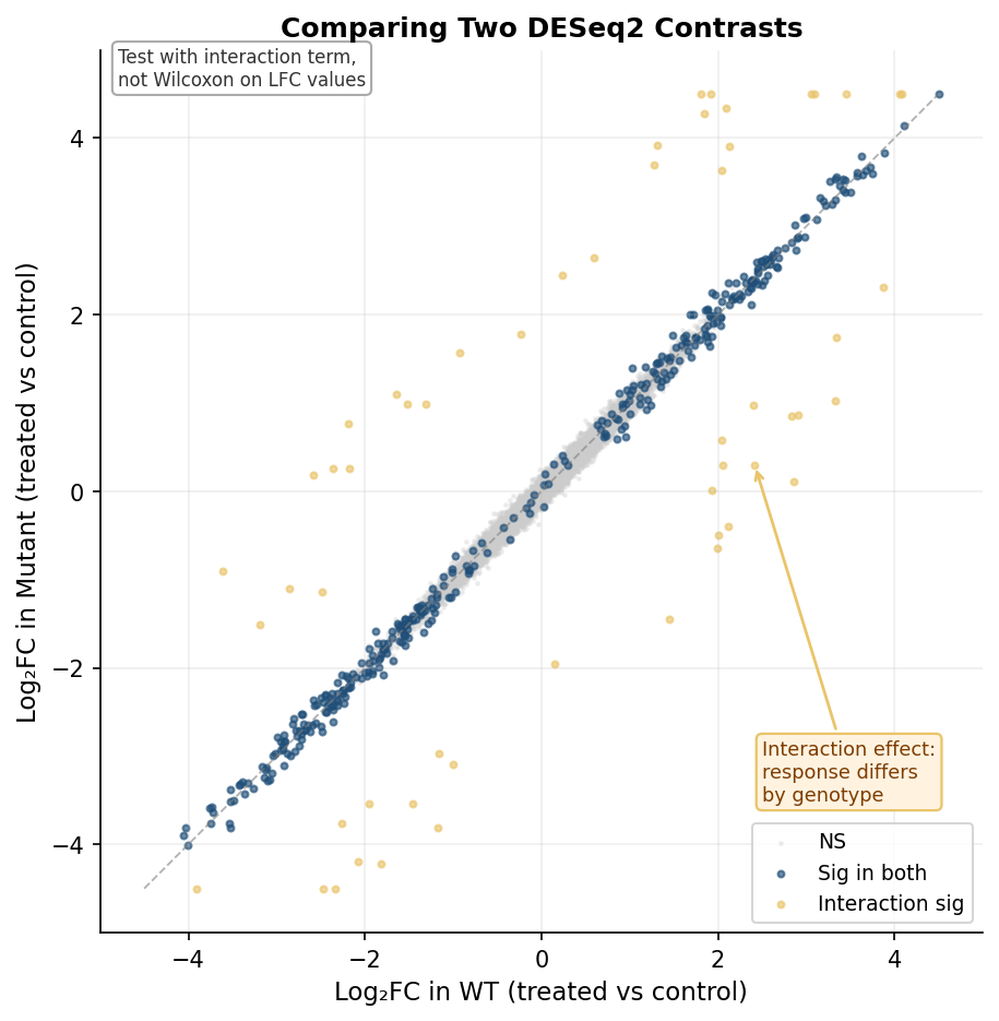
# What is the treatment effect specifically in mutants?# = main effect + interaction termres_treat_in_mut <- results(dds_interact, contrast = list(c("condition_treated_vs_control", "genotypemutant.conditiontreated")))Do not compare log2FC values between contrasts with a Wilcoxon test
A common mistake is extracting the log2FoldChange column from two separate DESeq2 results tables and running a Wilcoxon rank-sum test to ask whether the fold changes differ between the two contrasts. This is wrong for two reasons. First, the log2FC values across genes within one contrast are not independent observations drawn from a common distribution. Second, DESeq2 already models the uncertainty in each estimate; ignoring that uncertainty and treating estimated fold changes as if they were raw measurements discards the statistical framework you built the analysis on. The correct approach for comparing the magnitude of an effect across two conditions is to include an interaction term in the design formula and test the interaction coefficient directly.
The Combined Factor Shortcut
For complex designs where every pairwise comparison between multi-factor groups is needed, Mike Love’s recommended approach is to combine the factors into a single composite factor before building the DESeqDataSet. This sidesteps the interaction term algebra entirely and makes every comparison explicit via contrast.
# Combine genotype and condition into one factormetadata$group <- factor(paste(metadata$genotype, metadata$condition, sep = "_"))# Levels: "WT_control", "WT_treated", "mutant_control", "mutant_treated"
dds_combined <- DESeqDataSetFromMatrix(  countData = counts_matrix,  colData   = metadata,  design    = ~ 0 + group    # ~ 0 suppresses the intercept; each level gets its own coef)dds_combined <- DESeq(dds_combined)resultsNames(dds_combined)# "groupWT_control", "groupWT_treated", "groupmutant_control", "groupmutant_treated"
# Any comparison now specified by subtracting coefficient namesres_treat_WT  <- results(dds_combined,  contrast = list("groupWT_treated", "groupWT_control"))
res_treat_mut <- results(dds_combined,  contrast = list("groupmutant_treated", "groupmutant_control"))
# Interaction (is treatment effect different in mutants vs WT)?res_interact  <- results(dds_combined,  contrast = list(c("groupmutant_treated", "groupWT_control"),                  c("groupWT_treated",     "groupWT_control")))
This approach is less elegant mathematically but far easier to reason about. Every comparison is spelled out explicitly. There is no ambiguity about what each coefficient represents.
Case 4: Time-Course Designs
For experiments measuring gene expression at multiple timepoints, the analysis goal is usually to find genes that change across time, not genes that differ between any two specific timepoints. The likelihood ratio test (LRT) is the right tool.
# Metadata: subject ID and timepoint (T0, T2, T6, T24)metadata$timepoint <- factor(metadata$timepoint,                              levels = c("T0", "T2", "T6", "T24"))metadata$subject   <- factor(metadata$subject)
# For a paired time-course (same subjects at each timepoint):# Full model includes subject to account for repeated measuresdds_tc <- DESeqDataSetFromMatrix(  countData = counts_matrix,  colData   = metadata,  design    = ~ subject + timepoint)dds_tc <- DESeq(dds_tc, test = "LRT", reduced = ~ subject)
# LRT tests: does including timepoint significantly improve the model?# Genes with significant LRT padj changed at any point in the time courseres_tc <- results(dds_tc)
The LRT compares a full model (~ subject + timepoint) against a reduced model (~ subject) and identifies genes for which the timepoint term contributes significant explanatory power. A significant LRT result means the gene’s expression changes somewhere across the time course, but does not tell you where. Follow up with pairwise contrasts at specific timepoints to determine the pattern.
# Follow-up: pairwise contrasts at specific timepoints of interest# These use the same dds_tc object, just with results() for specific pairsres_T2_vs_T0 <- results(dds_tc, contrast = c("timepoint", "T2", "T0"))res_T24_vs_T0 <- results(dds_tc, contrast = c("timepoint", "T24", "T0"))Contrast Specification Cheat Sheet
| Design scenario | Formula | How to get contrast |
|---|---|---|
| Two conditions | ~ condition | results(dds, name = "condition_B_vs_A") |
| Three conditions, A vs control | ~ condition | results(dds, name = "condition_A_vs_control") |
| Three conditions, A vs B (non-ref) | ~ condition | results(dds, contrast = c("condition", "A", "B")) |
| Paired design | ~ subject + condition | results(dds, name = "condition_after_vs_before") |
| Two factors, additive | ~ genotype + condition | results(dds, name = "condition_treated_vs_control") |
| Two factors, interaction | ~ genotype + condition + genotype:condition | results(dds, name = "genotypeX.conditionY") |
| Combined factor | ~ 0 + group | results(dds, contrast = list("groupA", "groupB")) |
| Time course (any change) | ~ subject + timepoint, LRT | DESeq(dds, test = "LRT", reduced = ~ subject) |
| Time course, specific pair | ~ subject + timepoint (same dds) | results(dds, contrast = c("timepoint", "T6", "T0")) |
Common Mistakes and How to Avoid Them
Reversing the formula order. The factor of interest must be the last term. ~ condition + subject models condition as the primary effect and adjusts for subject. ~ subject + condition models subject as the primary effect and adjusts for condition. Only the second is correct for a paired design where you want the condition effect.
Forgetting to set the reference level. If you do not explicitly set levels on your factor, R uses alphabetical order. “treatA” comes before “control” alphabetically, which puts “control” as a non-reference level and inverts the direction of your fold changes. Always call factor(..., levels = c("control", "treatA", ...)) with control first.
Running separate DESeq2 analyses and comparing results. Running one DESeq2 on WT samples and another on mutant samples, then comparing their DEG lists or fold changes, is not equivalent to a proper interaction test. Size factor estimation and dispersion modeling will differ between the two runs, making the estimates incomparable. Always model all samples together with a design formula that captures the relevant factors.
Using Wald test for time courses. The Wald test at each timepoint answers “is gene X different at T6 vs T0?” The LRT answers “does gene X change at any point across the time course?” For discovery of time-responsive genes, the LRT is the appropriate test. Use pairwise Wald contrasts for follow-up characterization of genes already identified by LRT.
NotchBio validates your design matrix automatically before runs proceed. If the specified formula produces a rank-deficient model, the run is blocked with a specific error message identifying which column is causing the problem. The contrast builder pre-populates the available resultsNames() coefficients and generates the correct contrast syntax for non-reference comparisons, catching the most common multi-factor specification mistakes before they produce wrong results silently.
Related Reading
Further reading
Read another related post
FASTQ Quality Control with FastQC, fastp, and MultiQC
Bulk RNA-seq QC end to end: run FastQC on raw reads, trim adapters with fastp, rerun QC, and aggregate everything into one MultiQC report, with parallel runs.
TutorialDownload RNA-Seq Data from GEO and SRA with sra-tools
Download bulk RNA-seq FASTQ files from GEO and SRA: prefetch, fasterq-dump, pysradb metadata, batch downloads, and fixes for the most common errors.
TutorialHow to Make Volcano and MA Plots in R with ggplot2
Publication-quality volcano and MA plots from DESeq2 results in R: ggplot2 from scratch, ggrepel gene labels, EnhancedVolcano, and how to read them.