Batch Effect Correction Tools: ComBat-Seq vs RUVSeq vs sva
A batch effect is any systematic difference in measured gene expression that comes from technical factors rather than biological ones. Samples processed in different labs, on different days, with different RNA extraction kits, at different sequencing depths, or by different operators can all carry batch effects. When a batch effect is correlated with your condition of interest, it is indistinguishable from your biology. When it is not correlated, it adds noise that reduces your statistical power to detect real differences.
The good news is that most batch effects are detectable before you run differential expression analysis. The PCA plot is your first and most powerful diagnostic. The strategies for handling batch effects once detected are well-established and vary depending on whether the batch source is known, whether the batch is confounded with your condition, and whether you need corrected count matrices for downstream analysis.
This post focuses on choosing among the correction tools — ComBat-Seq, RUVSeq, and sva — including the harder case where the batch source is unknown or unmeasured, plus how to report correction in your methods section. If you are earlier in the process, What Are Batch Effects in RNA-Seq (and Why They Ruin Results) covers the concepts and Detecting Batch Effects with PCA and Correcting Them in DESeq2 walks through detection and the first-line design-covariate fix.
Spotting a Batch Effect on a PCA Plot
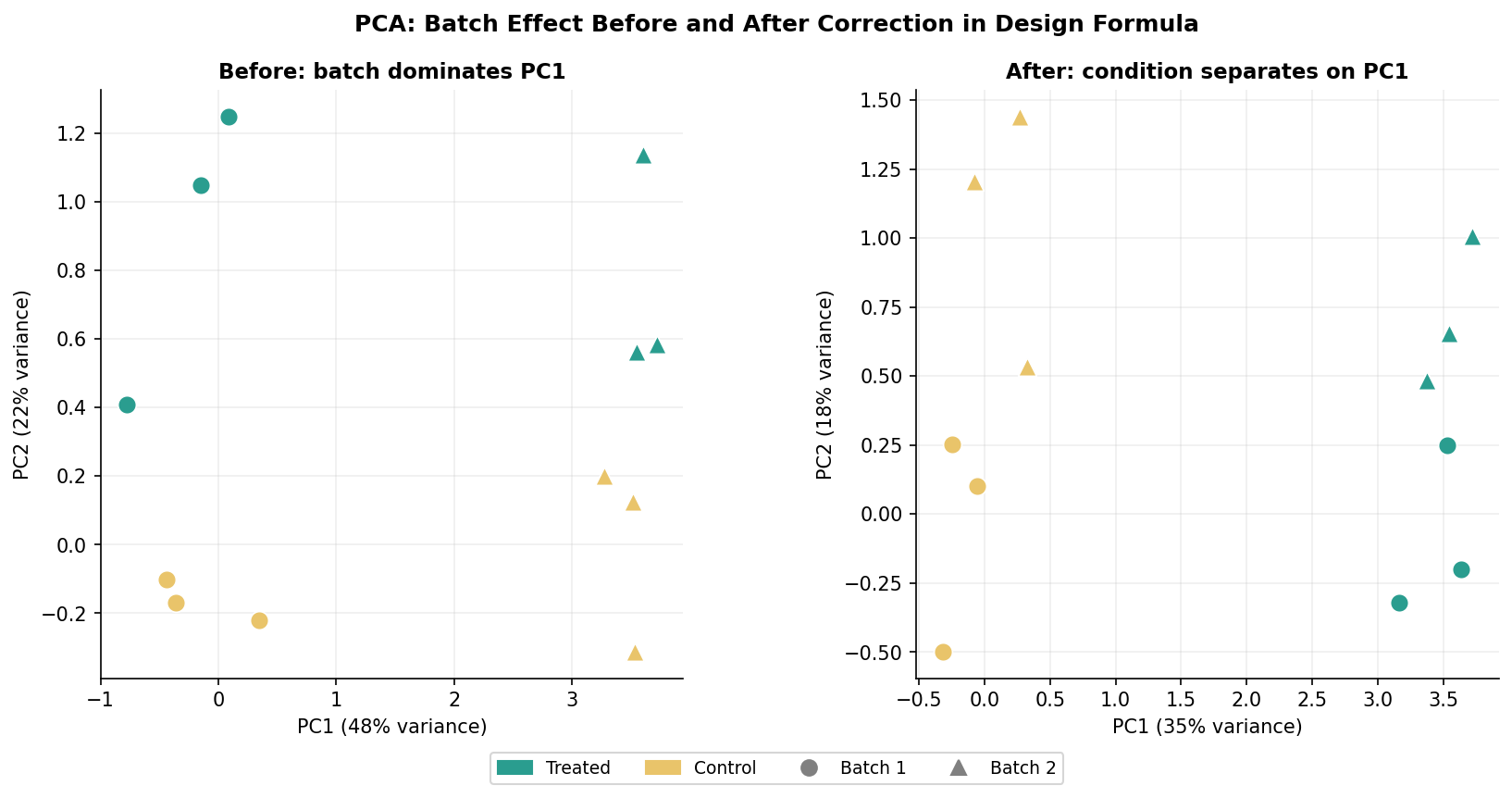
The PCA plot of normalized counts is the standard first-pass diagnostic for batch effects. If your samples separate primarily by condition along PC1, you have clean data. If they separate by batch along PC1 and by condition along PC2 or not at all, you have a batch effect that requires attention.
library(DESeq2)library(ggplot2)
# Build and normalize your DESeqDataSet (before running DESeq())dds <- DESeqDataSetFromMatrix(  countData = counts_matrix,  colData   = metadata,  design    = ~ condition)
# Variance-stabilizing transformation for PCAvsd <- vst(dds, blind = TRUE)   # blind = TRUE: do not use design info
# PCA with DESeq2's built-in functionpca_data <- plotPCA(vsd, intgroup = c("condition", "batch"),                    returnData = TRUE)
# Proportion of variance explained by each PCpercent_var <- round(100 * attr(pca_data, "percentVar"))
# Plot colored by condition AND shaped by batchggplot(pca_data, aes(PC1, PC2, color = condition, shape = batch)) +  geom_point(size = 4) +  xlab(paste0("PC1: ", percent_var[1], "% variance")) +  ylab(paste0("PC2: ", percent_var[2], "% variance")) +  theme_minimal() +  labs(title = "PCA: before batch correction")
Two patterns signal a batch effect. The first is when samples cluster by batch rather than by condition on the first two PCs. The second, subtler pattern is when the variance explained by PC1 is very high (above 60 to 70 percent) and is driven by a technical covariate rather than biology. Check both by coloring the PCA by condition and batch separately and comparing.
The First-Line Fix: Batch as a Design Covariate
If your batch is known and is not completely confounded with your condition (every sample in batch 1 is treated, every sample in batch 2 is control), the correct first response is to include batch as a covariate in your DESeq2 design formula. This is the statistically cleanest approach and requires no external tools.
# Include batch in the design formula# Rule: factor of interest (condition) must be LAST in the formulametadata$batch     <- factor(metadata$batch)metadata$condition <- factor(metadata$condition, levels = c("control", "treated"))
dds <- DESeqDataSetFromMatrix(  countData = counts_matrix,  colData   = metadata,  design    = ~ batch + condition   # batch first, condition last)
dds <- DESeq(dds)
# Extract the condition effect, statistically adjusted for batchres <- results(dds, name = "condition_treated_vs_control")
This approach tells DESeq2 to estimate and account for systematic differences between batches while estimating the condition effect. The returned fold changes and p-values reflect the biological comparison you care about, with batch variation partitioned out of the residuals.
The one case where this approach fails is confounding: if every sample in batch 1 is treated and every sample in batch 2 is control, batch and condition are perfectly correlated. The model matrix becomes rank-deficient and DESeq2 will raise an error. In this case there is no statistical solution: the batch and condition effects cannot be separated. The experiment needs to be redesigned.
When the Design Covariate Is Not Enough: ComBat-Seq
Including batch in the design formula handles batch effects at the statistical level but does not change the count matrix itself. If you need batch-corrected counts for visualization, for sharing with collaborators, or for input to tools that do not accept design formulas, you need a count-level correction tool.
ComBat-Seq by Zhang et al. (2020) is the appropriate tool for RNA-seq count data. It uses negative binomial regression to model and remove batch effects while preserving the integer nature of counts, making the output compatible with DESeq2 and edgeR. The original ComBat used a Gaussian model appropriate for microarray intensities but not for count data. ComBat-Seq specifically addresses this.
Never use ComBat-Seq corrected counts as input to DESeq2 for DE analysis
ComBat-Seq produces batch-adjusted counts that are useful for visualization and for tools that do not accept design formulas. However, using ComBat-Seq corrected counts as the countData input to DESeq2 and then also including batch in the design formula double-corrects for the batch effect and inflates your false discovery rate. The correct workflow is: use ComBat-Seq corrected counts for PCA and heatmap visualization, and use the original uncorrected counts with batch in the design formula for differential expression analysis.
# Install ComBat-Seq via sva packageif (!requireNamespace("sva", quietly = TRUE)) {  BiocManager::install("sva")}library(sva)
# counts_matrix must be a genes-by-samples integer matrix# batch is a vector of batch labels matching the column order of counts_matrixadjusted_counts <- ComBat_seq(  counts    = as.matrix(counts_matrix),  batch     = metadata$batch,  group     = metadata$condition,  # preserve biological signal for this group  full_mod  = TRUE                 # use full model; recommended)
# adjusted_counts is now a batch-corrected integer matrix# Use it ONLY for visualization; use original counts for DESeq2 DE analysis
# PCA after ComBat-Seq correctiondds_viz <- DESeqDataSetFromMatrix(  countData = adjusted_counts,  colData   = metadata,  design    = ~ condition)vsd_viz <- vst(dds_viz, blind = TRUE)plotPCA(vsd_viz, intgroup = c("condition", "batch"))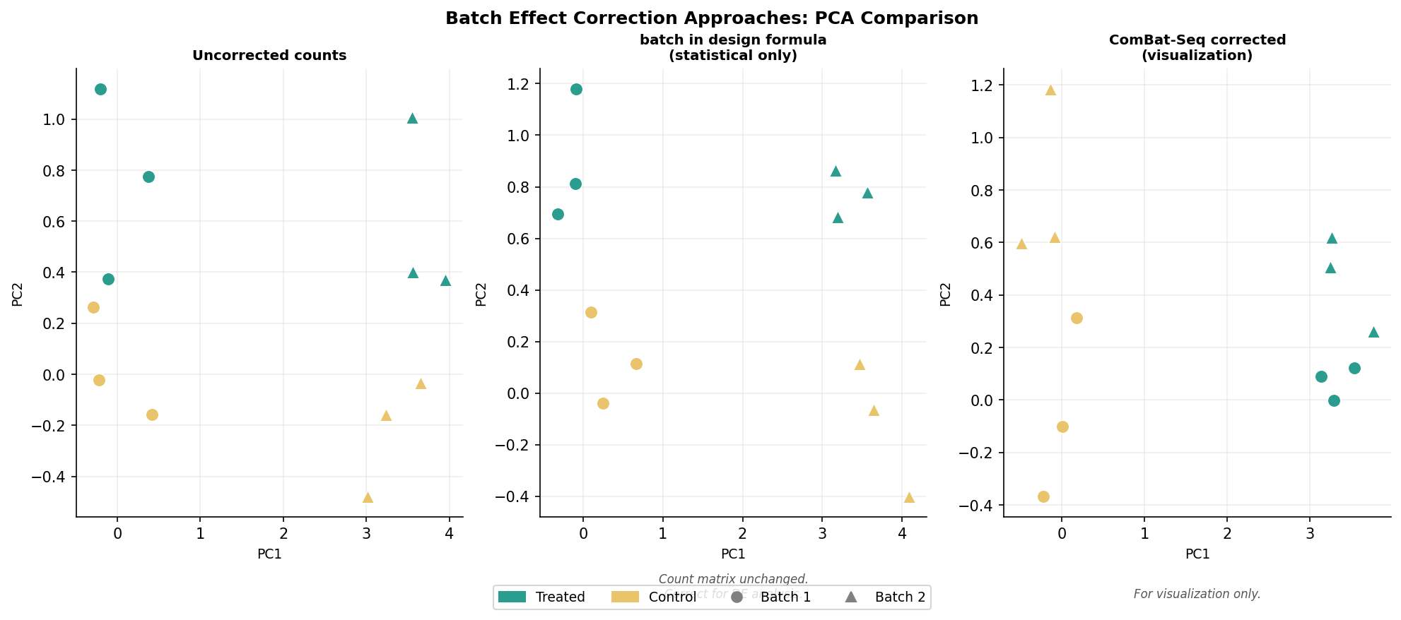
RUVSeq and sva: When the Batch Source Is Unknown
Sometimes you know samples were processed differently but you do not have a recorded batch variable. Maybe the lab rotation student who processed samples three and four used a slightly different protocol. Maybe there was a freeze-thaw cycle that affected some samples. Principal components analysis will tell you something is wrong, but you do not have a label to put in the design formula.
RUVSeq (remove unwanted variation from RNA-Seq data) by Risso et al. (2014) estimates factors of unwanted variation from the data itself, using one of three approaches. RUVg uses control genes known not to change between conditions (housekeeping genes or ERCC spike-ins) to estimate technical factors. RUVs uses replicate samples to estimate factors. RUVr uses residuals from a first-pass GLM.
The sva package by Leek (2014) takes a similar approach using surrogate variable analysis. It identifies components of variation in the expression data that are not explained by your primary biological variable and estimates them as surrogate variables.
library(RUVSeq)
# Option 1: RUVg with empirical controls# (genes least significant in a first-pass DE analysis serve as controls)dds_firstpass <- DESeqDataSetFromMatrix(  countData = counts_matrix,  colData   = metadata,  design    = ~ condition)dds_firstpass <- DESeq(dds_firstpass)res_firstpass <- results(dds_firstpass)
# Genes not significantly DE in the first pass are candidate control genesempirical_controls <- rownames(res_firstpass)[  which(res_firstpass$padj > 0.5 & !is.na(res_firstpass$padj))]
# Build a SeqExpressionSet for RUVSeqx_condition <- factor(metadata$condition)set <- newSeqExpressionSet(  as.matrix(counts_matrix),  phenoData = data.frame(x_condition,                          row.names = colnames(counts_matrix)))
# Estimate k=1 factor of unwanted variation using empirical controlsset1 <- RUVg(set, empirical_controls, k = 1)
# W_1 is the estimated unwanted variation factor# Include it in the DESeq2 design formulametadata$W1 <- pData(set1)$W_1
dds_ruv <- DESeqDataSetFromMatrix( countData = counts_matrix, colData = metadata, design = ~ W1 + condition # W1 as batch surrogate, condition last)dds_ruv <- DESeq(dds_ruv)res_ruv <- results(dds_ruv, name = "condition_treated_vs_control")library(sva)
# sva approach: estimate surrogate variables# mod: full model with condition; mod0: null model without conditionmod <- model.matrix(~ condition, data = metadata)mod0 <- model.matrix(~ 1, data = metadata)
# Estimate surrogate variables from log-normalized countsnorm_counts <- log1p(counts(estimateSizeFactors( DESeqDataSetFromMatrix(counts_matrix, metadata, ~ condition)), normalized = TRUE))
svobj <- sva(norm_counts, mod, mod0)
# Add surrogate variables to metadata and DESeq2 designfor (i in seq_len(svobj$n.sv)) { metadata[[paste0("SV", i)]] <- svobj$sv[, i]}
sv_terms <- paste0("SV", seq_len(svobj$n.sv))design_formula <- as.formula(paste("~", paste(c(sv_terms, "condition"), collapse = " + ")))
dds_sva <- DESeqDataSetFromMatrix( countData = counts_matrix, colData = metadata, design = design_formula)dds_sva <- DESeq(dds_sva)res_sva <- results(dds_sva, name = "condition_treated_vs_control")The choice between RUVSeq and sva depends largely on what control information you have. If you have ERCC spike-ins or a confirmed set of housekeeping genes, RUVg is more powerful because the control gene set is biologically motivated. If you have no controls, sva or RUVr are the alternatives. In practice the results are similar for datasets where the unwanted variation is moderate.
Reporting Batch Correction in the Methods
Your methods section must state which approach you used and why. The phrasing differs depending on the method:
For the design formula approach: “Batch effects were accounted for by including the batch assignment as a covariate in the DESeq2 design formula (~ batch + condition). Differential expression results reflect the condition effect adjusted for between-batch variability.”
For ComBat-Seq used for visualization: “ComBat-Seq (Zhang et al., 2020, NAR Genomics and Bioinformatics) was applied to batch-adjusted count matrices for visualization purposes. Differential expression analysis was performed on the original uncorrected counts with batch included as a covariate in the DESeq2 design formula.”
For RUVSeq or sva: “Surrogate variables (or: factors of unwanted variation) were estimated from the count data using RUVSeq (Risso et al., 2014) with k=1 factors and included as covariates in the DESeq2 design formula. The number of factors was selected by PCA inspection of the corrected data.”
Which Tool for Which Situation
| Situation | Recommended approach | Use ComBat-Seq? | Notes |
|---|---|---|---|
| Batch known, not confounded with condition | batch in design formula | For visualization only | Statistically cleanest; always try this first |
| Batch known, confounded with condition | No statistical fix | N/A | Must redesign experiment; any result is unreliable |
| Need batch-corrected counts for a collaborator | ComBat-Seq | Yes | Keep original counts for your own DE analysis |
| Batch known, need counts for non-DESeq2 tools | ComBat-Seq | Yes | Preserves integer counts unlike limma removeBatchEffect |
| Batch unknown, have ERCC spike-ins | RUVSeq::RUVg | No | Use spike-ins as control genes |
| Batch unknown, have replicates | RUVSeq::RUVs or sva | No | Add estimated factors to design formula |
| Batch unknown, no controls | sva | No | Estimate from data; treat as exploratory |
NotchBio automatically generates the PCA colored by every metadata column present in your sample table and flags samples where a non-condition variable explains more variance than condition on the first two PCs. When the platform detects that batch and condition are confounded, it blocks the analysis and raises a warning explaining why the result would be statistically uninterpretable. For datasets with a valid batch covariate, the batch term is included in the DESeq2 design formula automatically.
Related Reading
Further reading
Read another related post
FASTQ Quality Control with FastQC, fastp, and MultiQC
Bulk RNA-seq QC end to end: run FastQC on raw reads, trim adapters with fastp, rerun QC, and aggregate everything into one MultiQC report, with parallel runs.
TutorialDownload RNA-Seq Data from GEO and SRA with sra-tools
Download bulk RNA-seq FASTQ files from GEO and SRA: prefetch, fasterq-dump, pysradb metadata, batch downloads, and fixes for the most common errors.
TutorialHow to Make Volcano and MA Plots in R with ggplot2
Publication-quality volcano and MA plots from DESeq2 results in R: ggplot2 from scratch, ggrepel gene labels, EnhancedVolcano, and how to read them.