Cell Line Pathway Analysis: Methods and Comparisons
Cell line pathway analysis tests whether coordinated gene programs differ between cell lines, respond to treatment, or respond differently in one line than another.
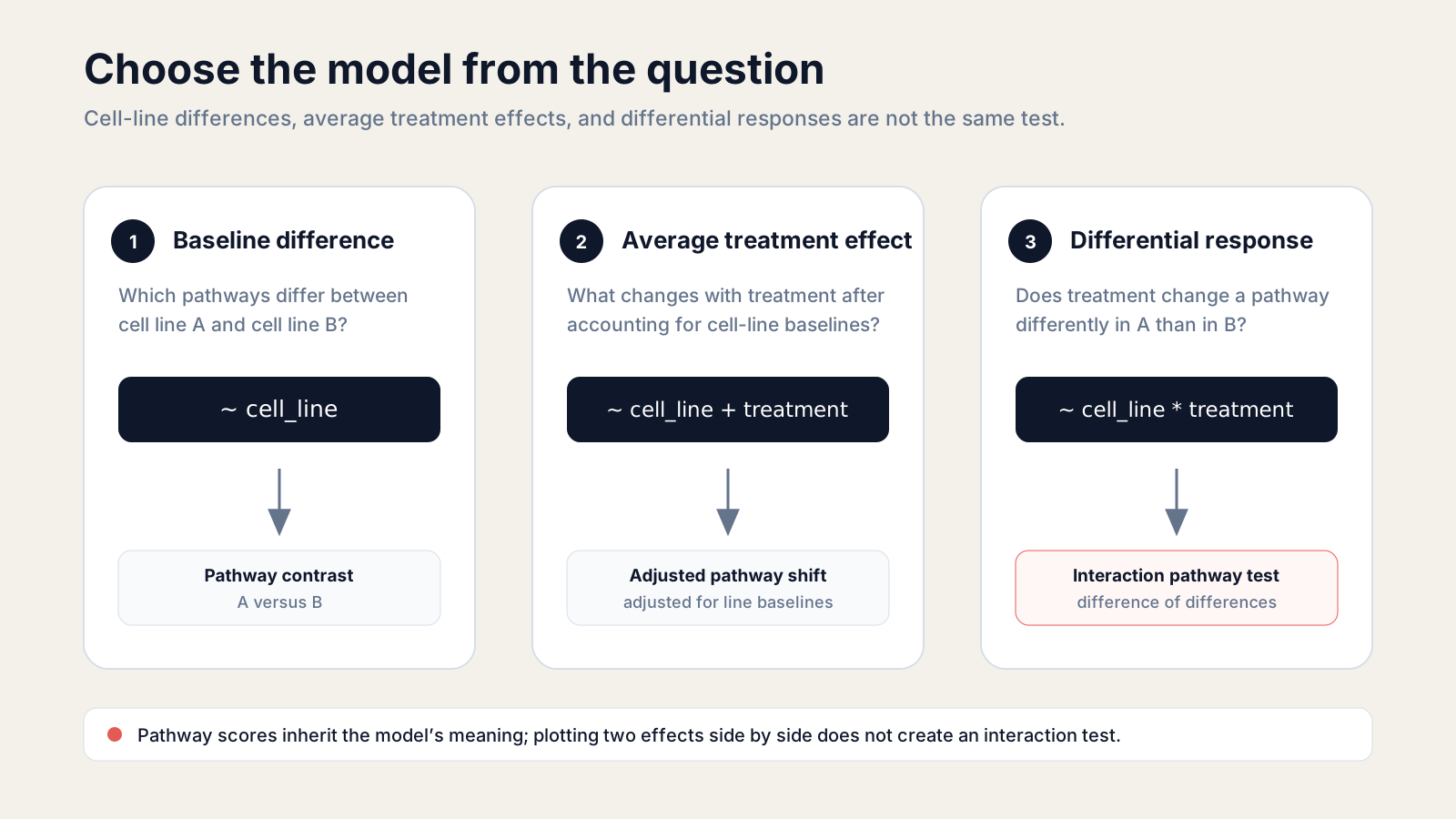
The correct pathway method starts with the experimental question and RNA-seq design. A baseline contrast, an adjusted treatment effect, and a treatment-by-cell-line interaction estimate different quantities. No pathway plot can repair a model that tests the wrong one.
This guide shows how to select the model, derive pathway evidence, compare lines on a common scale, and interpret the result without turning association into mechanism.
What is cell line pathway analysis?
Cell line pathway analysis summarizes gene-level evidence into curated pathways or regulator footprints while preserving the cell-line comparison defined by the RNA-seq model.
The measured input is usually a gene-level statistic from differential expression: a Wald statistic, shrunken log2 fold change, or signed significance score. The pathway layer then asks whether members are overrepresented, shifted in a ranking, or consistent with a signed model.
These evidence layers answer different questions. Enrichment detects coordinated membership or rank shifts. Topology propagates change through signed, directed edges. Activity inference compares measured target behavior with a weighted prior network.
A member-expression heatmap is useful supporting evidence, but it is not a pathway-activation score. Likewise, co-expression between genes does not establish a regulatory edge.
The unit of inference remains the biological replicate. Wells split from one culture are technical replicates, not independent evidence about cell-line response. The companion guide on cell line RNA-seq design failures covers authentication, passage drift, contamination, and pseudoreplication.
Which cell-line question are you testing?
Choose one estimand before choosing a pathway database: baseline difference, treatment effect within or across lines, or differential treatment response between lines.
| Question | Example RNA-seq design | Gene-level quantity sent to pathways |
|---|---|---|
| Do lines differ at baseline? | ~ cell_line | line A versus line B |
| Is there an average treatment effect? | ~ cell_line + treatment | treatment coefficient adjusted for line |
| Does treatment response differ by line? | ~ cell_line * treatment | interaction coefficient |
| What is treatment response within each line? | combined-factor or stratified model | one treatment contrast per line |
The baseline model compares stable transcriptional differences between lines. Its pathways may reflect tissue of origin, genotype, differentiation state, culture adaptation, or unmeasured laboratory history. They do not describe treatment response.
The additive model asks for a treatment effect after accounting for cell-line baselines. It assumes the treatment effect being estimated is shared in the modeled sense. It does not estimate how much the effect changes from one line to another.
The interaction model asks a difference-of-differences question. For two lines and two treatment states, it tests whether treated − control in line B differs from treated − control in line A.
Write the intended coefficient in words before collecting data. “The treatment effect in B minus the treatment effect in A” exposes the required four groups and prevents a baseline contrast from being mislabeled as response specificity.
With more than two lines, choose planned interaction contrasts rather than treating every possible pair as equally important. Pre-specification reduces interpretive drift and limits the number of gene- and pathway-level questions multiplied across the study.
The official DESeq2 vignette documents multi-factor designs, interaction coefficients, combined-factor designs, and the need to inspect resultsNames(dds) before extracting a result.
How many biological replicates do you need?
Use at least three independent biological replicates per cell-line-by-condition group as a practical starting point, then justify the final number with power, variance, and effect-size assumptions.
Two replicates can make a simple model technically estimable, but they provide fragile dispersion estimates and little protection against an outlier. More complex designs require enough independent samples in every combination represented by the interaction.
For a 3-line × 2-treatment experiment with three replicates per combination, the design has 18 biological samples. Three wells from the same flask still count as one biological event, even if each well receives a separate library.
Power depends on sequencing depth, dispersion, expected effect, multiplicity, and balance. Adding depth cannot substitute for independent replication once counts are sufficient to estimate expression reliably.
Balance matters as much as count. If all line A samples are processed in batch 1 and all line B samples in batch 2, cell line and batch are perfectly confounded. No additive formula can identify which factor produced the difference.
Randomize culture, extraction, library preparation, and sequencing across conditions when possible. Record passage, serum lot, operator, plate, and processing date before analysis so suspected nuisance variables are not reconstructed from memory.
Replicates must support the interaction
An interaction needs observations in each cell-line-by-treatment combination. A missing group, single replicate, or perfectly confounded batch can make the design non-estimable or too unstable for a credible pathway comparison.
Should cell line be a group or blocking variable?
Make cell line the primary variable when lines are the comparison; use it as an additive blocking variable when another factor is primary and baseline line differences are nuisance variation.
With ~ cell_line, DESeq2 produces line-to-line gene contrasts. Ranked pathway analysis on each contrast answers which programs are shifted between lines under the sampled condition.
With ~ cell_line + treatment, the treatment coefficient is adjusted for baseline differences among lines. This can improve precision when the additive assumption is defensible and the design is balanced.
Cell line is not a conventional random block when each named line is itself scientifically important. In the additive formula, it is a fixed-effect factor included to absorb systematic baseline differences.
If the scientific goal is a response for each line, encode each line-treatment combination as one factor or fit planned within-line contrasts. The DESeq2 vignette presents the combined-factor approach as a practical way to retrieve specific group comparisons.
Separate stratified models are easier to explain but discard information sharing across lines and can produce different filtering or dispersion behavior. A combined model usually gives a cleaner basis for formal comparisons when its assumptions hold.
Blocking also requires overlap. If every treatment level is absent from one line, the adjusted treatment coefficient depends on extrapolation or becomes non-estimable. Make a sample-by-factor table and inspect the design matrix before fitting counts.
For continuous covariates such as passage number, preserve the recorded numeric value when the assumed relationship is meaningful. Turning passage into arbitrary bins can discard information, but assuming a linear effect without diagnostics can also mislead.
When do you need a treatment-by-cell-line interaction?
Use an interaction when the claim is that treatment changes a gene or pathway differently across cell lines, not merely that one line passes FDR and another does not.
For a two-factor design, ~ cell_line + treatment + cell_line:treatment is equivalent to ~ cell_line * treatment. The interaction coefficient measures the extra treatment effect for a non-reference line relative to the reference line.
library(DESeq2)
# Set the biological reference levels before fitting.samples$cell_line <- relevel(factor(samples$cell_line), ref = "A")samples$treatment <- relevel(factor(samples$treatment), ref = "control")stopifnot(nlevels(samples$cell_line) == 2)stopifnot(nlevels(samples$treatment) == 2)
dds <- DESeqDataSetFromMatrix(  countData = counts,  colData = samples,  design = ~ cell_line * treatment)
dds <- DESeq(dds)resultsNames(dds)
# Names depend on factor levels; select the intended interaction explicitly.interaction_name <- grep(  "cell_line.*treatment|treatment.*cell_line",  resultsNames(dds),  value = TRUE)stopifnot(length(interaction_name) == 1)interaction <- results(dds, name = interaction_name)
The interaction statistic can be ranked for pathway analysis. A positive pathway score then means member genes tend toward a more positive treatment response in line B than line A, subject to the chosen gene-set method.
That language is comparative, not absolute. A positive interaction can occur when both lines increase but B increases more, when A decreases and B increases, or when A decreases more strongly than B.
Use a Wald test for a specific interaction coefficient. A likelihood-ratio test can ask whether one or more interaction terms improve the model by comparing a full design with a reduced additive design, but its result is an omnibus test and does not supply one signed effect by itself.
For pathway ranking, a signed, coefficient-specific statistic is easier to interpret than an unsigned omnibus p-value. If the omnibus test is primary, follow it with planned coefficients or contrasts before assigning a direction to a pathway.
Do not test interaction by comparing two significance labels. “Significant in A, nonsignificant in B” does not imply that A and B differ significantly. The interaction directly tests the difference between effects.
The original DESeq2 paper explains the negative-binomial model, dispersion estimation, shrinkage, and multiple-testing framework beneath these coefficients.
How do you compare pathways across cell lines?
Compare complete, harmonized pathway score tables on a shared scale, preserving direction, uncertainty, pathway version, measured size, and missingness.
Start from one model and one pathway collection when possible. Use stable pathway identities, the same gene universe, the same organism mapping, and the same ranking rule across line-specific contrasts.
Thresholded hit lists are a poor comparison unit. A pathway with FDR 0.049 in line A and 0.051 in line B may be nearly identical, while two significant pathways can have opposite effects.
Keep effect and significance separate. A tidy comparison table should include pathway, collection, contrast, score, fdr, measured_size, leading_edge, and evidence_type.
Choose the pathway method from the input contract. ORA can annotate an interaction-DEG list but is sensitive to the cutoff. Ranked analysis retains the full interaction statistic. Activity inference tests whether weighted targets follow a regulator model.
Run multiple-testing correction within a clearly defined family and report that family. A line-specific table, an interaction table, and several pathway collections can create many hypotheses; silently selecting the most favorable view defeats the stated FDR.
Missing results must remain missing. A pathway may be unavailable because too few genes were measured, identifiers failed to map, the collection changed, or a signed topology graph was unavailable. None of those states equals a score of zero.
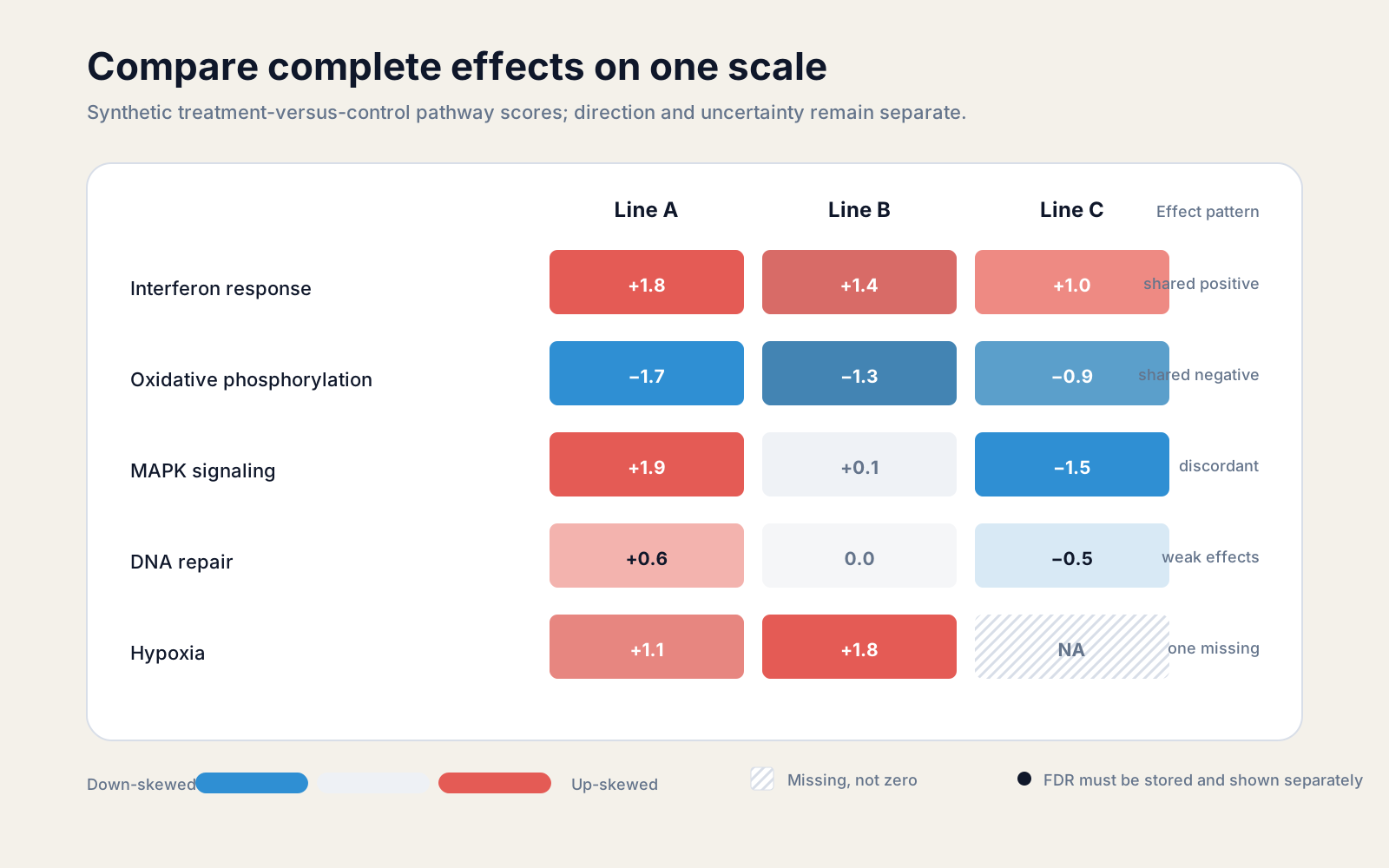
For descriptive agreement, report Spearman correlation across complete scores, sign agreement, and the largest discordant pathways. For inference about differential response, use the interaction-derived gene statistic rather than correlation between two pathway tables.
When datasets were fitted separately, harmonize gene identifiers and pathway releases before joining. Cross-study score comparisons need additional treatment of platform, batch, and study uncertainty; they are not interchangeable with contrasts from one fitted experiment.
How should baseline expression differences be handled?
Model baseline line differences at the gene level, then interpret pathway scores from the resulting contrast rather than subtracting pathway plots after analysis.
Cell lines can differ in copy number, lineage programs, mutations, growth rate, and media dependence. The Cancer Cell Line Encyclopedia demonstrated why molecular profiles and drug responses vary substantially across large cell-line panels.
Baseline expression affects both detectability and interpretation. A pathway may have fewer measurable members in one line, creating weaker coverage even when the biological response is comparable.
Inspect normalized counts for driver genes, but do not use normalized counts as the input to DESeq2. Differential testing starts from raw integer counts, while transformations such as VST are for visualization and quality assessment.
Authentication is part of the statistical contract. Cellosaurus records cell-line identities, synonyms, and problematic lines, while its CLASTR service supports STR-profile similarity searches.
Passage number, mycoplasma, media, confluence, and serum lot can also alter baseline programs. Include a nuisance factor only when the design contains enough independent, non-confounded observations to estimate it.
Which plots reveal shared and cell-line-specific responses?
Use PCA for sample structure, an effect matrix for pathway comparison, gene-level plots for drivers, and shared-scale trajectories only when the condition order is meaningful.
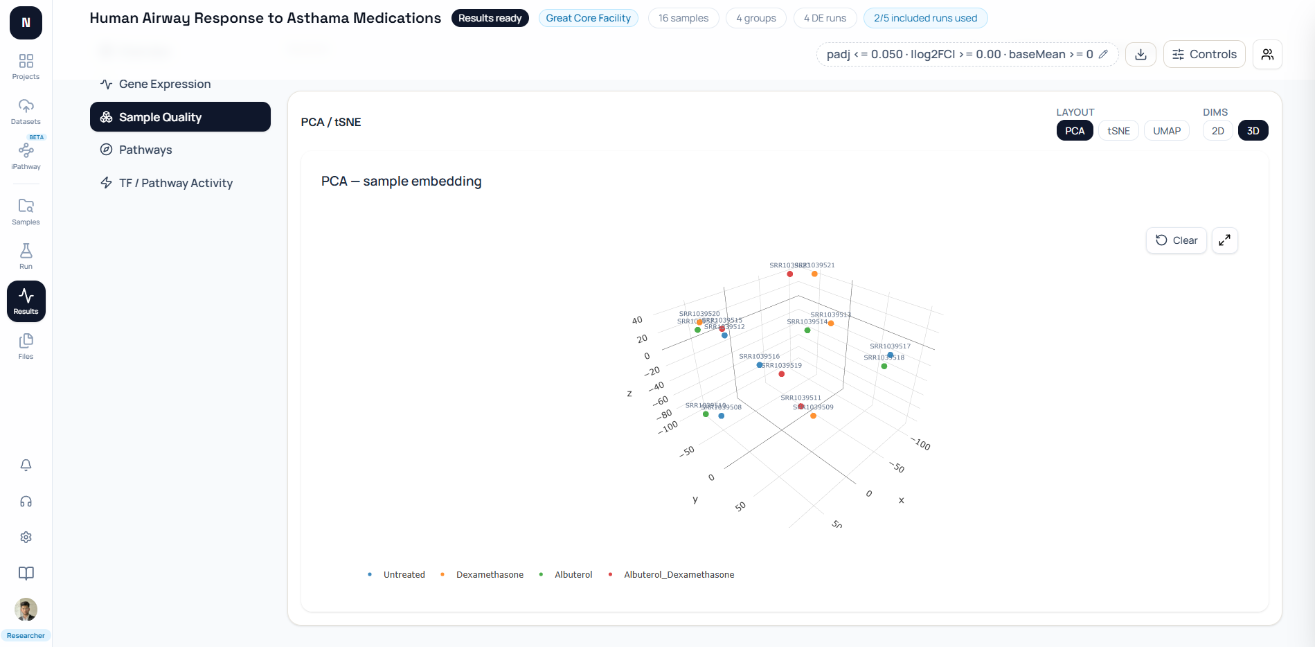
PCA is a diagnostic, not a treatment test. It can reveal separation by cell line, treatment, or batch, but axes summarize variance and visible clusters do not establish causality.
A pathway-by-contrast matrix is the central comparison view. Use a common zero-centered scale, encode direction with a diverging palette, and show FDR or uncertainty through a separate mark rather than color intensity alone.
A gene-level multi-contrast table identifies whether one pathway score is driven by the same genes in every line. It also reveals sign reversals hidden by a single set-level summary.
A barcode or running-sum view shows where pathway members fall in each ranked gene list. A leading-edge table then identifies which members drive the set-level shift and whether the drivers recur across lines.
Show uncertainty when the method provides it. Confidence intervals for gene coefficients, FDR for pathway tests, measured-gene coverage, and sensitivity to pathway collection are more informative than a grid of significance stars.
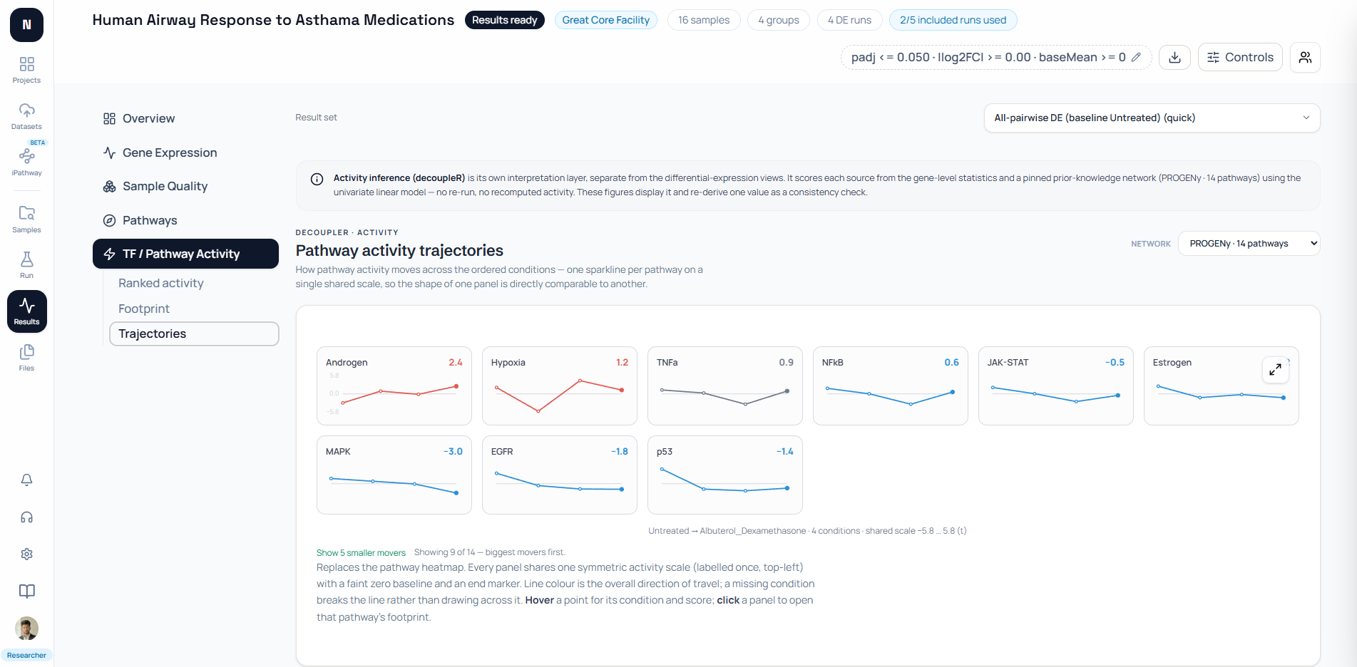
Pathway trajectories are appropriate for ordered doses, time points, or a biologically justified sequence. Do not connect unrelated treatment groups with a line merely because the plotting library expects an order.
How does NotchBio model cell line today?
NotchBio currently supports cell line as a primary or additive blocking variable and builds pairwise contrasts for the primary variable; it does not expose interaction terms in the run interface.
The run configuration defines three design variables: group, cell_line, and batch. Its formula builder places selected blocking variables before the primary variable, producing formulas such as ~ cell_line + group.
The run interface checks that every sample has values for the primary and blocking variables. It requires at least two primary levels, flags levels below two samples, and recommends three or more samples per level.
On the backend, NotchBio writes the selected terms into sample metadata, converts them to factors, and passes the additive formula to DESeq2. It then generates planned pairwise contrasts across levels of the primary variable.

That behavior supports baseline line comparisons when cell_line is primary. It also supports treatment comparisons adjusted for cell line when group is primary and cell_line is additive.
It does not test whether treatment response differs by line. For that claim, fit ~ cell_line * treatment in a workflow that exposes interactions, then run pathway analysis on the interaction statistic or on explicit within-line treatment contrasts.
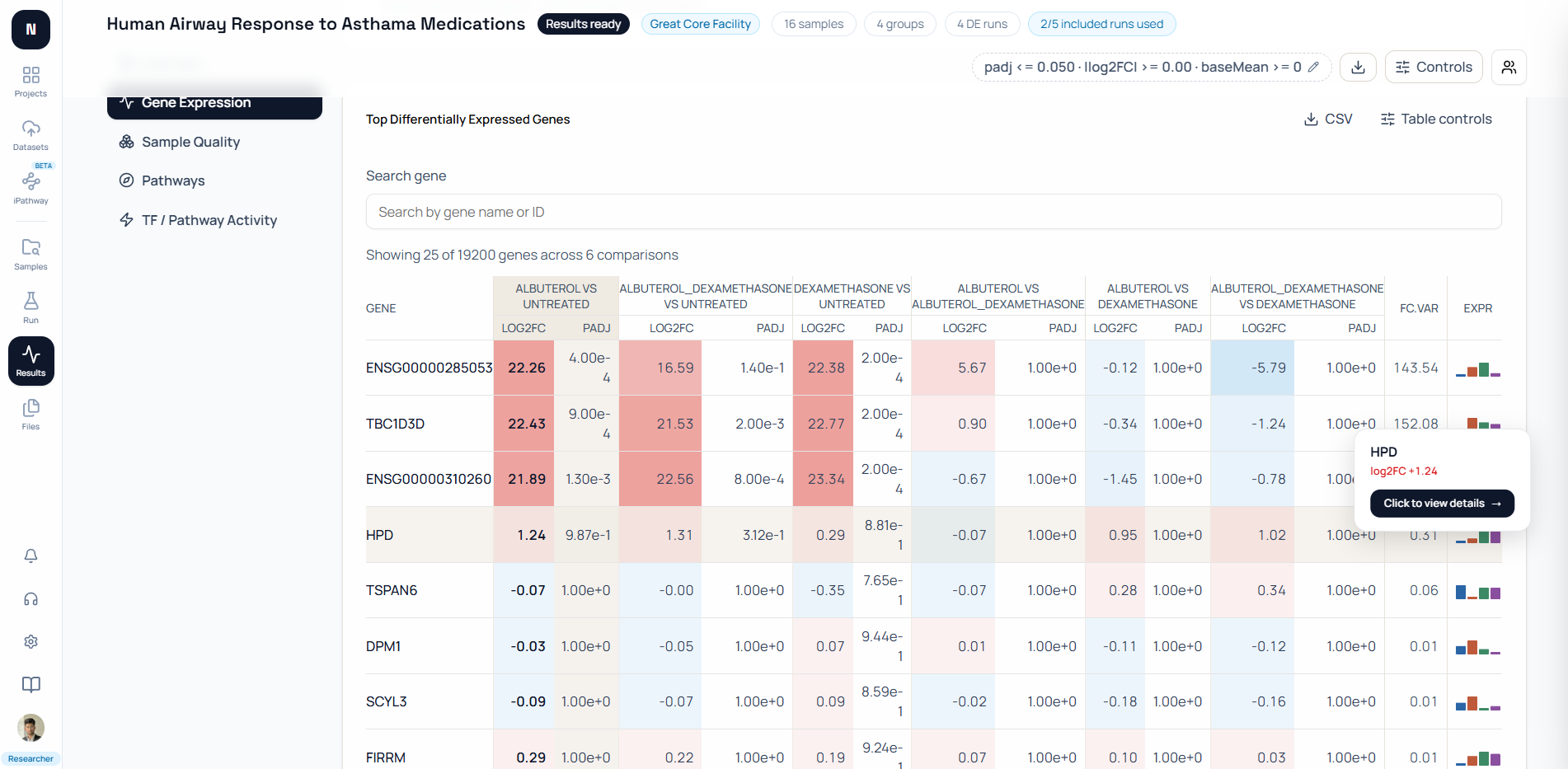
The Results Pathways workspace coordinates enrichment, topology, member-gene, and activity views for a selected comparison. It keeps directional enrichment separate from topology-based predicted activation or inhibition.
This product boundary is deliberate in this article: the current screenshot catalog lacks an approved capture of the cell-line design selector, so Figure 6 proves pairwise-baseline semantics only. The behavior described above is grounded in current source code, not inferred from that image.
What should be validated experimentally?
Validate cell identity, the driver genes behind the pathway score, and the predicted phenotype with an orthogonal assay before making a mechanistic claim.
First, confirm identity with current STR profiling and check the line against a reference resource. Test for mycoplasma and record passage, media, serum, confluence, and treatment timing.
Second, inspect the leading-edge or high-weight genes. Confirm that their expression changes are consistent, well covered, and not carried by one outlier sample.
Third, match validation to the evidence layer. Use targeted RNA or protein assays for member changes, phosphoproteomics or biochemical readouts for signaling state, and a functional assay for the phenotype.
Choose the assay before reading the most exciting pathway name. A predeclared readout reduces the temptation to validate only a convenient downstream marker that is shared by many unrelated programs.
Rescue, inhibition, or perturbation experiments are needed to strengthen causal claims. Enrichment, co-expression, topology propagation, and activity inference are structured hypothesis generators, not substitutes for intervention.
Finally, reproduce the response in independent biological replicates and, when generalization matters, in another relevant line or model. A result replicated within one immortalized line is evidence about that system, not automatically about a tumor, tissue, or patient population.
The next practical step is to pair this design logic with multiple-condition DESeq2 contrasts and a full pathway enrichment workflow. For sample-level diagnostics, use the RNA-seq PCA guide.
To align results across lines, studies, or platforms, use How to Compare Pathways Across Datasets. Then turn the comparison table into honest figures with Pathway Visualization in Python.
Further reading
Read another related post
PyDESeq2 vs DESeq2 in R: Validation and Scanpy Workflow
Does PyDESeq2 really match R DESeq2? A tutorial on validating results against R, running PCA with scanpy and AnnData, and exporting DEGs for enrichment.
BioinformaticsReproducible RNA-Seq Pipelines: Versions, Tools, and Provenance
Run snapshots, version pinning, and locked parameters should be the default, not a feature. A practitioner case for reproducibility-first RNA-seq platforms.
TutorialPublication-Ready RNA-Seq Plots in R with ggplot2
Reviewer-ready RNA-seq plots in R: volcano with gene labels, z-score heatmap with annotation bars, PCA with variance explained, and journal export settings.