Pathway Enrichment Analysis: GSEA and ORA in R and Python
A list of 1,200 differentially expressed genes is not a result. It is raw material.
Without pathway context, you cannot answer the biological question your experiment was designed to address. Is the treatment activating an inflammatory response? Suppressing a metabolic pathway? Inducing an epithelial-to-mesenchymal transition? Pathway enrichment analysis answers these questions by testing whether biologically coherent gene sets are systematically shifted in your data.
This tutorial covers two complementary approaches: Gene Set Enrichment Analysis (GSEA), which uses the full ranked gene list, and Over-Representation Analysis (ORA), which tests a significant DEG list against a background. Both are implemented in R with clusterProfiler and in Python with gseapy. We use the results from Blog 7 and Blog 8 as input.
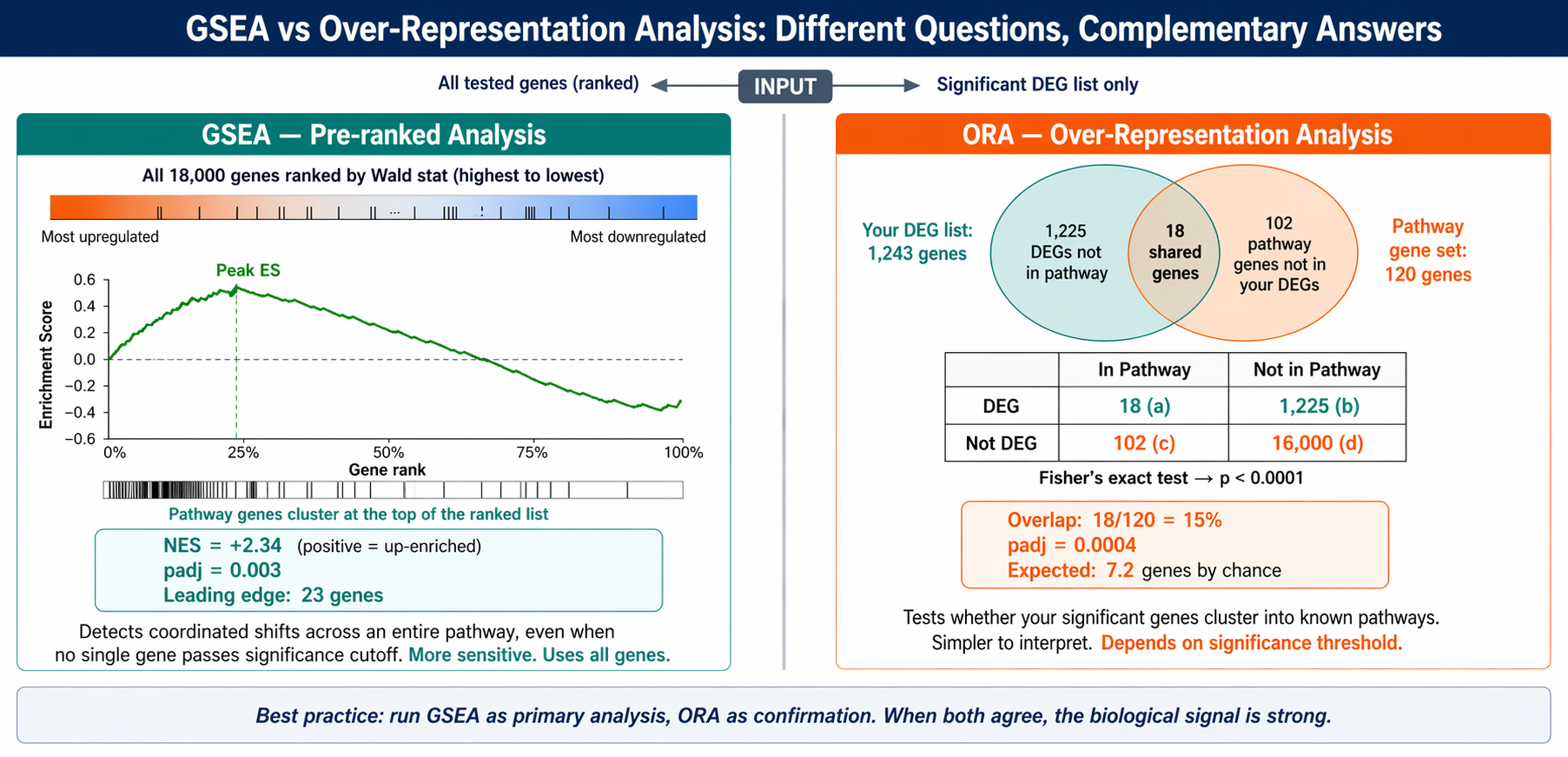
GSEA vs ORA: Which One to Use
People often run both and report whichever gives more impressive results. That is not the right approach.
GSEA requires no significance threshold. It uses every gene in your experiment, ranked by a continuous metric. It is more sensitive to subtle, coordinated shifts across a pathway. It is the preferred method when you want to capture changes in biological processes, not just the loudest individual genes.
ORA requires a defined DEG list. It asks whether the genes you called significant happen to cluster into known pathways more than random chance would predict. It is faster to interpret but loses information about genes just below the significance threshold. Use it when your DEG list has clear biological meaning you want to annotate.
In practice, GSEA with the full ranked list is the primary analysis. ORA on the significant DEGs is a useful complement for generating pathway hypotheses.
Which ranking metric to use for GSEA
The Wald test statistic (the stat column in DESeq2 results) is a better ranking metric than log2 fold change alone. It encodes both effect size and statistical confidence because it is the fold change divided by its standard error. Genes with large, well-supported fold changes rank higher than genes with large but noisy fold changes. Always use stat for ranking when it is available.
How to Run GSEA in R with clusterProfiler and MSigDB Hallmark Gene Sets
Install required packages
# Install onceBiocManager::install(c("clusterProfiler", "enrichplot", "org.Hs.eg.db"))install.packages("msigdbr")Load the packages and results
library(clusterProfiler)library(enrichplot)library(msigdbr)library(org.Hs.eg.db)library(ggplot2)library(dplyr)library(readr)
# Load DESeq2 results from Blog 5res <- read_csv("results/deseq2/all_genes.csv") |>  filter(!is.na(stat), !is.na(symbol))
Build the ranked gene list
# Use the Wald stat as ranking metric# Strip version numbers from Ensembl IDsres <- res |>  mutate(gene_id_clean = sub("\\..*", "", gene_id))
# Map Ensembl IDs to Entrez IDs# clusterProfiler needs Entrez for most MSigDB lookupsid_map <- bitr(  res$gene_id_clean,  fromType = "ENSEMBL",  toType   = "ENTREZID",  OrgDb    = org.Hs.eg.db)
res_mapped <- res |>  left_join(id_map, by = c("gene_id_clean" = "ENSEMBL")) |>  filter(!is.na(ENTREZID)) |>  distinct(ENTREZID, .keep_all = TRUE)
# Named numeric vector: names = Entrez IDs, values = Wald statranked_list <- res_mapped$statnames(ranked_list) <- res_mapped$ENTREZIDranked_list <- sort(ranked_list, decreasing = TRUE)
cat("Ranked list length:", length(ranked_list), "\n")# Typically 15,000-19,000 genes with Entrez mappings
Fetch MSigDB Hallmark gene sets
# MSigDB Hallmark gene sets: 50 curated pathways# Each represents a specific biological state or processh_gene_sets <- msigdbr(species = "Homo sapiens", category = "H") |>  dplyr::select(gs_name, entrez_gene) |>  dplyr::rename(ont = gs_name, gene = entrez_gene)
# Alternatively, use C2 (KEGG, Reactome, Biocarta):# c2_gene_sets <- msigdbr(species = "Homo sapiens", category = "C2")
# Or GO Biological Processes:# c5_gene_sets <- msigdbr(species = "Homo sapiens", category = "C5", subcategory = "BP")
cat("Hallmark gene sets loaded:", length(unique(h_gene_sets$ont)), "\n")# 50 pathways
Run GSEA
set.seed(2024)
gsea_result <- GSEA(  geneList     = ranked_list,  TERM2GENE    = h_gene_sets,  minGSSize    = 15,      # minimum genes in a set after filtering  maxGSSize    = 500,     # maximum genes per set  pvalueCutoff = 0.05,  pAdjustMethod = "BH",  eps          = 0,       # more precise p-values (slower but important)  seed         = TRUE,  verbose      = FALSE)
# View significant pathwaysas.data.frame(gsea_result) |>  arrange(p.adjust) |>  dplyr::select(ID, NES, pvalue, p.adjust, setSize, core_enrichment) |>  head(10)
The key columns in the output are NES (normalized enrichment score), p.adjust (BH-corrected p-value), and core_enrichment (the leading edge genes).
A positive NES means the pathway is enriched in the up-regulated direction. A negative NES means enrichment in the down-regulated direction.
What NES means and what it does not mean
The normalized enrichment score corrects for gene set size, so you can compare NES values across pathways with different numbers of genes. However, you cannot meaningfully compare NES values across different experiments or different gene set collections. Always report both NES and the adjusted p-value. Never rank pathways by NES alone.
Visualize with dotplot and ridgeplot
library(enrichplot)
# Dotplot of top enriched pathwaysp_dot <- dotplot(  gsea_result,  showCategory = 15,  x            = "NES",  color        = "p.adjust",  size         = "setSize",  label_format = 40) +  scale_color_gradient(low = "#0D9488", high = "#F97316",                       name = "Adjusted p") +  labs(title = "GSEA: MSigDB Hallmark (Treated vs Control)") +  theme_minimal(base_size = 11)
ggsave("results/figures/gsea_dotplot.pdf",       p_dot, width = 8, height = 7, dpi = 300, device = "pdf")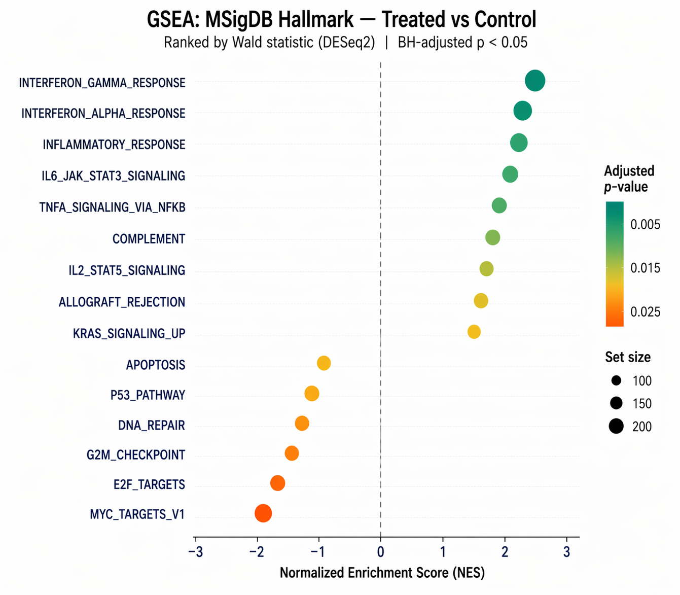
How to Run Over-Representation Analysis (ORA) with enrichGO
ORA tests whether a list of significant genes is enriched for specific GO terms compared to the background of all tested genes.
# Significant DEGs onlysig_genes <- res_mapped |>  filter(padj < 0.05, abs(log2FoldChange) > 1) |>  pull(ENTREZID)
# Background: all genes that were tested (not just significant ones)background_genes <- res_mapped$ENTREZID
cat("Significant DEGs for ORA:", length(sig_genes), "\n")cat("Background genes:", length(background_genes), "\n")
# Run GO Biological Process over-representation analysisora_result <- enrichGO(  gene          = sig_genes,  universe      = background_genes,  OrgDb         = org.Hs.eg.db,  ont           = "BP",        # Biological Process; use "MF" or "CC" for others  pvalueCutoff  = 0.05,  pAdjustMethod = "BH",  qvalueCutoff  = 0.2,  readable      = TRUE         # converts Entrez IDs to gene symbols in output)
# Simplify redundant GO termsora_simple <- simplify(ora_result, cutoff = 0.7, by = "p.adjust")
# View top resultsas.data.frame(ora_simple) |>  arrange(p.adjust) |>  dplyr::select(Description, GeneRatio, BgRatio, p.adjust, geneID) |>  head(10)
Always provide a background gene list for ORA
The default background in enrichGO() is all genes in the organism database, which is around 20,000 for human. Your actual background should be the genes you actually tested, not all genes that exist. If you only measured 15,000 genes due to low-count filtering, using all 20,000 as background overstates statistical significance. Always set universe = background_genes explicitly.
How to Run GSEA in Python with gseapy
GSEApy is a comprehensive Python package for gene set enrichment analysis. Its core is written in Rust for performance, and it provides six tools: gsea for full GSEA, prerank for pre-ranked lists, ssgsea for single sample GSEA, enrichr for over-representation analysis, and several others.
Install it if you have not already:
pip install gseapyBuild the ranked gene list
import pandas as pdimport numpy as npimport gseapy as gp
# Load PyDESeq2 results from Blog 6res = pd.read_csv("results/pydeseq2/all_genes.csv", index_col=0)res = res.dropna(subset=["stat", "symbol"])
# Use Wald statistic for ranking# The stat column in PyDESeq2 matches the stat column in R DESeq2ranked = (    res[["symbol", "stat"]]    .dropna()    .drop_duplicates(subset="symbol", keep="first")    .sort_values("stat", ascending=False)    .set_index("symbol")["stat"])
print(f"Ranked list length: {len(ranked)}")print(ranked.head())# IFNG    18.43# STAT1   16.72# IRF1    15.89# ISG15   14.34# IFIT1   13.91
Run pre-ranked GSEA with Hallmark gene sets
# gseapy can pull gene sets directly from MSigDB or Enrichr# No need to download GMT files manually
gsea_result = gp.prerank(    rnk           = ranked,    gene_sets     = "MSigDB_Hallmark_2020",   # fetches from Enrichr automatically    threads       = 4,    min_size      = 15,    max_size      = 500,    permutation_num = 1000,    outdir        = "results/gsea_prerank",    seed          = 2024,    verbose       = False)
# Access the results DataFrameresult_df = gsea_result.res2d.sort_values("FDR q-val")print(result_df[["Term","NES","NOM p-val","FDR q-val","Lead_genes"]].head(10))
Available gene set libraries you can pass as a string include: "MSigDB_Hallmark_2020", "KEGG_2021_Human", "Reactome_2022", "GO_Biological_Process_2023". The library name is passed to the Enrichr API and the current list can be retrieved with gp.get_library_name().
Visualize the enrichment score plot for one pathway
# Enrichment plot for a specific pathwayterms = gsea_result.res2d.Term.tolist()
# Find the most significant pathwaytop_term = result_df.iloc[0]["Term"]
ax = gp.gseaplot(    rank_metric  = gsea_result.ranking,    term         = top_term,    **gsea_result.results[top_term],    figsize      = (6, 4))ax[0].figure.savefig("results/figures/gsea_enrichment_plot.pdf",                     dpi=300, bbox_inches="tight")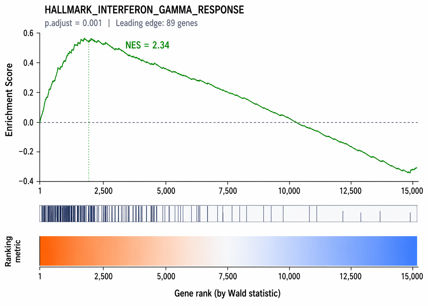
How to Run ORA in Python with gseapy.enrichr
ORA in Python does not require a ranked list. Pass your significant gene symbols directly to gseapy.enrichr.
# Significant DEG symbolssig_symbols = (    res.query("padj < 0.05 and abs(log2FoldChange) > 1")    ["symbol"]    .dropna()    .tolist())print(f"ORA input: {len(sig_symbols)} significant genes")
# Run ORA against GO Biological Process and Hallmarkenr_result = gp.enrichr(    gene_list     = sig_symbols,    gene_sets     = ["GO_Biological_Process_2023", "MSigDB_Hallmark_2020"],    organism      = "human",    outdir        = "results/ora_enrichr",    cutoff        = 0.05)
# Access resultsenr_df = enr_result.results.sort_values("Adjusted P-value")print(enr_df[["Gene_set","Term","Overlap","Adjusted P-value","Genes"]].head(10))
Unlike GSEA, enrichr hits the Enrichr web API and returns results within seconds. An internet connection is required.
Export and summarize results
# Save all enrichment results to CSVresult_df.to_csv("results/gsea_prerank/gsea_hallmark_results.csv", index=False)enr_df.to_csv("results/ora_enrichr/ora_results.csv",    index=False)
# Quick dotplot with gseapyax = gp.dotplot(    gsea_result.res2d,    column     = "FDR q-val",    title      = "GSEA: MSigDB Hallmark",    cmap       = "RdYlGn_r",    size       = 6,    top_term   = 15,    figsize    = (6, 8))ax.figure.savefig("results/figures/gsea_dotplot_python.pdf",                  dpi=300, bbox_inches="tight")
Comparing GSEA and ORA Results
Running both methods together gives you a more complete picture.
GSEA captures gradual shifts in pathway activity that may not reach the DEG threshold. A pathway where 80 of its 120 genes show modest but consistent up-regulation will score well in GSEA but have no genes in your DEG list at padj < 0.05.
ORA captures the pathways most concentrated in your strongest DEGs. If five of your top 20 significant genes are interferon-stimulated genes, ORA flags interferon signaling even if the pathway is not strongly enriched across the entire ranked list.
| Comparison dimension | GSEA | ORA |
|---|---|---|
| Input | Full ranked gene list (all tested genes) | Significant DEG list only |
| Ranking metric | Wald stat, log2FC, or any continuous score | Not applicable |
| Threshold sensitivity | None: uses all genes | Depends heavily on padj/LFC cutoffs |
| Best for | Detecting coordinated pathway shifts | Annotating your significant hit list |
| Reference sets | MSigDB Hallmark, KEGG, Reactome, GO | Same sets |
| Key output | NES, leading edge genes | Overlap, p-value, gene list |
| R implementation | clusterProfiler::GSEA(), fgsea::fgsea() | clusterProfiler::enrichGO() |
| Python implementation | gseapy.prerank() | gseapy.enrichr() |
| Recommended background | N/A: all genes are used | All tested genes, not the organism genome |
A practical workflow is to run GSEA first to identify which biological themes are systematically perturbed, then use ORA to confirm those themes in your high-confidence DEG list. When the two methods agree, that is strong evidence. When they disagree, it usually means either your significance cutoff is too stringent for the pathway signal you are chasing, or a single outlier gene is driving the ORA result.
Manual Enrichment Pipeline vs NotchBio
Running enrichment analysis end-to-end takes around an hour: bitr mapping for Entrez IDs, choosing between GSEA and ORA, downloading the right MSigDB collection, tuning the min/max gene set sizes, and generating the dotplots.
NotchBio runs both GSEA and ORA automatically as part of every differential expression report. Results include Hallmark, KEGG, Reactome, and GO Biological Process for each comparison.
| Step | Manual (R or Python) | NotchBio |
|---|---|---|
| Install clusterProfiler / gseapy | BiocManager + conda, 5-10 min | Not required |
| Map gene IDs | bitr() in R, mygene in Python | Automatic |
| Build ranked list | Sort by stat, handle NA, deduplicate | Automatic |
| Fetch gene sets | msigdbr() or Enrichr API | Pre-loaded for human, mouse, rat |
| Run GSEA | GSEA() or gseapy.prerank() | Automatic for Hallmark, KEGG, GO |
| Run ORA | enrichGO() or gseapy.enrichr() | Automatic |
| Simplify redundant terms | simplify() or manual filtering | Automated term clustering |
| Generate dotplots | dotplot() + ggsave() at 300 dpi | Included in report |
| Export results | Manual CSV exports | Download from dashboard |
| Time to enrichment results | 45-90 min | 5 min after DE analysis |
If you want pathway enrichment results without managing Bioconductor package installs or Enrichr API calls, notchbio.app runs the full GSEA and ORA pipeline as part of every differential expression analysis.
Further reading
Read another related post
How to Run STAR Alignment for Bulk RNA-Seq (Step-by-Step)
Complete STAR alignment tutorial: download genome and GTF, build a genome index with the right sjdbOverhang, run paired-end alignment, generate GeneCounts, and load counts into R for DESeq2.
TutorialHow to Build a Salmon Index and Quantify Bulk RNA-Seq Reads
Step-by-step Salmon tutorial: download GENCODE references, build a decoy-aware index, run salmon quant with gcBias and seqBias on all samples, and verify mapping rates before DESeq2.
TutorialHow to Run FASTQ Quality Control with FastQC, fastp, and MultiQC
Full pipeline tutorial for bulk RNA-seq QC: run FastQC on raw reads, trim adapters with fastp, rerun QC, and aggregate reports with MultiQC. Includes parallel processing and how to read results.