Bulk RNA-Seq Deconvolution: CIBERSORTx and MuSiC Tutorial
Bulk RNA-seq averages gene expression across every cell in your sample. If you are studying a tumor biopsy, that average mixes cancer cells, fibroblasts, endothelial cells, and infiltrating immune cells in proportions that vary between patients. If you are studying a tissue biopsy before and after treatment, a change in measured expression might reflect altered gene regulation, or it might reflect a shift in which cell types are present. Deconvolution computationally separates these contributions by comparing your bulk expression profile against a reference describing what each cell type looks like.
This tutorial covers the two most widely used deconvolution tools: CIBERSORTx, which uses a signature matrix derived from sorted cells or single-cell data, and MuSiC, which uses a multi-subject single-cell reference and is implemented in R. Both produce estimates of cell type proportions per sample. Understanding when to use each and how to validate the output is as important as running the tool.
When Deconvolution Is the Right Answer
Deconvolution answers a specific question: what fraction of each bulk sample is composed of each cell type? It is the right choice when you have bulk RNA-seq data from a heterogeneous tissue and want to ask whether the proportions of specific cell types differ between your conditions.
Deconvolution is not a replacement for single-cell RNA-seq. It cannot identify transcriptional states within a cell type. It cannot detect rare populations present in fewer than roughly 5 percent of cells. It cannot tell you how an individual cell behaves. What it can tell you, at bulk RNA-seq cost, is whether the immune infiltrate in your tumor differs between responders and non-responders, or whether fibroblast abundance changes with disease progression.
The method works best when the expected compositional differences between groups are relatively large, when a high-quality reference exists for your tissue and species, and when the cell types you care about are transcriptionally distinct. It becomes unreliable when the reference does not match your tissue context, when two cell types share most of their marker genes, or when the expected compositional shift is smaller than the method’s estimation error.
Choosing a Reference: The Most Important Decision
The choice of reference is the single biggest determinant of deconvolution accuracy. A reference built from blood immune cells will perform poorly on brain tissue. A reference built from healthy tissue will misattribute gene expression from disease-specific cell states.
The LM22 signature matrix bundled with CIBERSORTx is appropriate for immune deconvolution of blood and tumors but not for parenchymal tissue cell types. If you are deconvolving tumor samples, tissue-specific references built from paired single-cell and bulk RNA-seq data from the same cancer type consistently outperform generic immune references.
The reference must match your tissue and, ideally, your disease condition
Using a blood immune cell reference (like LM22) on non-blood tissue data is one of the most common deconvolution mistakes. For non-immune tissues, build or obtain a reference from single-cell RNA-seq data generated from the same tissue and, where possible, the same disease condition. A reference built from healthy tissue will misestimate cell type proportions in disease if condition-specific cell states differ substantially from the reference cell types. MuSiC2, the updated version of MuSiC, was specifically designed for this cross-condition mismatch problem.
Public reference resources worth checking before building your own:
- The Human Cell Atlas provides curated single-cell references for many tissues
- CellChat and CellTypist provide pre-trained classifiers that can be adapted for signature extraction
- The CIBERSORTx website hosts community-submitted signature matrices for specific tissues
- The Heart Cell Atlas and similar organ-specific atlases provide tissue-matched references for CIBERSORTx and MuSiC
CIBERSORTx Walkthrough
CIBERSORTx by Newman et al. (2019) is a web-based tool. Upload your bulk expression matrix and a signature matrix; it returns estimated cell type fractions for each sample. CIBERSORTx also offers a single-cell mode where you can upload raw scRNA-seq data and it will build the signature matrix automatically.
Preparing the Input Files
CIBERSORTx expects gene expression in CPM or TPM units, not raw counts. If you have a DESeq2 results object, you need the normalized count matrix rather than the raw counts:
library(DESeq2)
# Assume dds is your DESeqDataSet after estimateSizeFactors()# Get size-factor normalized countsnorm_counts <- counts(dds, normalized = TRUE)
# Convert to CPM (counts per million)# This is appropriate for CIBERSORTx inputcpm_matrix <- sweep(norm_counts, 2, colSums(norm_counts), "/") * 1e6
# Export as tab-separated file with gene names as first column# CIBERSORTx requires the first column to be named "GeneSymbol"cpm_df <- data.frame(  GeneSymbol = rownames(cpm_matrix),  cpm_matrix,  check.names = FALSE)
write.table(cpm_df,            "mixture_for_cibersortx.txt",            sep       = "\t",            row.names = FALSE,            quote     = FALSE)
If you are using the LM22 matrix for immune deconvolution, it is available for download after free registration on the CIBERSORTx website. For custom references from scRNA-seq data, upload the count matrix with cell type annotations and use the “Create Signature Matrix” module first.
Batch Correction Mode
CIBERSORTx offers two batch correction modes for when the reference and mixture data come from different platforms or protocols. B-mode (bulk mode) is appropriate when the signature matrix was built from bulk sorted cells or plate-based scRNA-seq. S-mode (single-cell mode) is appropriate when the signature matrix was built from droplet-based scRNA-seq (10x Genomics, Drop-seq). If your reference and mixture data were generated on the same platform, batch correction may not be necessary.
Parsing CIBERSORTx Results in R
library(ggplot2)library(tidyr)library(dplyr)
# Load CIBERSORTx output (downloaded from the website)deconv_results <- read.table(  "CIBERSORTx_Results.txt",  header    = TRUE,  sep       = "\t",  row.names = 1,  check.names = FALSE)
# Keep only the cell fraction columns (remove p-value, correlation, RMSE)fraction_cols <- setdiff(  colnames(deconv_results),  c("P-value", "Correlation", "RMSE"))fractions <- deconv_results[, fraction_cols]
# Add condition metadatafractions$sample    <- rownames(fractions)fractions$condition <- metadata[rownames(fractions), "condition"]
# Reshape for plottingfractions_long <- fractions |>  tidyr::pivot_longer(    cols      = all_of(fraction_cols),    names_to  = "cell_type",    values_to = "proportion"  )
# Stacked bar chart of cell type proportions per sampleggplot(fractions_long,       aes(x = sample, y = proportion, fill = cell_type)) +  geom_col(width = 0.8) +  scale_fill_brewer(palette = "Set3", name = "Cell type") +  labs(    x     = NULL,    y     = "Estimated proportion",    title = "Cell type composition by sample (CIBERSORTx)"  ) +  theme_classic(base_size = 10) +  theme(    axis.text.x = element_text(angle = 45, hjust = 1, size = 8),    legend.text = element_text(size = 7)  ) +  facet_grid(. ~ condition, scales = "free_x", space = "free_x")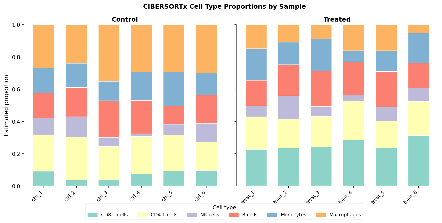
MuSiC Walkthrough
MuSiC by Wang et al. (2019, Nature Communications) is an R package that uses multi-subject scRNA-seq data as its reference. Its key advantage over CIBERSORTx is that it explicitly accounts for cross-subject variability in the single-cell reference, which reduces the bias that arises from using a single-donor reference for multi-donor bulk data.
Installing MuSiC
# Install devtools if neededif (!requireNamespace("devtools", quietly = TRUE))  install.packages("devtools")
# Install MuSiC from GitHub (includes MuSiC2)devtools::install_github("xuranw/MuSiC")
library(MuSiC)library(Biobase)          # for ExpressionSetlibrary(SingleCellExperiment)
Preparing the Reference
MuSiC requires the single-cell reference in ExpressionSet format with cell type annotations in the phenotype data:
# sc_counts: genes x cells integer count matrix from your scRNA-seq reference# sc_meta: data frame with columns: cell_id, cell_type, subject_id
sc_eset <- ExpressionSet(  assayData   = sc_counts,  phenoData   = new("AnnotatedDataFrame",                    data = sc_meta))
# Inspect the referencetable(pData(sc_eset)$cell_type)     # cell type distributiontable(pData(sc_eset)$subject_id)    # samples contributing cells
A high-quality MuSiC reference has at least 3 to 5 subjects contributing cells, at least 50 cells per cell type per subject, and cell types that are cleanly annotated with no ambiguous clusters. If your reference has fewer than 3 subjects, the cross-subject weighting that distinguishes MuSiC from simpler approaches provides little benefit.
Running Deconvolution
# bulk_eset: ExpressionSet of your bulk RNA-seq data (normalized counts)# Ensure gene names are consistent between bulk and single-cell reference
music_results <- music_prop(  bulk.mtx    = exprs(bulk_eset),       # genes x samples bulk matrix  sc.sce      = sc_eset,                # single-cell reference ExpressionSet  clusters    = "cell_type",            # column in sc pData for cell types  samples     = "subject_id",           # column in sc pData for subjects  select.ct   = NULL,                   # NULL = use all cell types in reference  verbose     = FALSE)
# Extract estimated proportionsestimated_props <- music_results$Est.prop.weighted
# Each row is a sample, each column is a cell typehead(estimated_props)
# Summary statistics by conditionprops_df <- as.data.frame(estimated_props)props_df$condition <- metadata[rownames(props_df), "condition"]
# Mean proportion per cell type per conditionprops_df |>  dplyr::group_by(condition) |>  dplyr::summarise(dplyr::across(where(is.numeric), mean)) |>  print()
Comparing CIBERSORTx and MuSiC Estimates
Running both tools on the same dataset and comparing their estimates is the most informative validation step. High concordance (Pearson r above 0.9 for major cell types) indicates the result is stable across methodologies. Low concordance for a specific cell type suggests that cell type’s estimated proportions are sensitive to modeling assumptions and should be treated cautiously.
# Merge estimates from both tools# ciber_props: CIBERSORTx proportions (samples x cell types)# music_props: MuSiC proportions (samples x cell types)
# Match cell types present in both (names may differ)shared_types <- intersect(colnames(ciber_props), colnames(music_props))
comparison_df <- data.frame(  sample    = rep(rownames(ciber_props), length(shared_types)),  cell_type = rep(shared_types, each = nrow(ciber_props)),  cibersort = as.vector(as.matrix(ciber_props[, shared_types])),  music     = as.vector(as.matrix(music_props[, shared_types])))
# Scatter plot: CIBERSORTx vs MuSiC estimatesggplot(comparison_df, aes(x = cibersort, y = music, color = cell_type)) +  geom_point(size = 2, alpha = 0.7) +  geom_abline(slope = 1, intercept = 0, linetype = "dashed", color = "grey50") +  facet_wrap(~ cell_type, scales = "free") +  labs(    x     = "CIBERSORTx proportion",    y     = "MuSiC proportion",    title = "Method concordance: CIBERSORTx vs MuSiC"  ) +  theme_classic(base_size = 9) +  theme(legend.position = "none")
# Compute per-cell-type concordanceconcordance <- comparison_df |>  dplyr::group_by(cell_type) |>  dplyr::summarise(pearson_r = cor(cibersort, music, method = "pearson")) |>  dplyr::arrange(desc(pearson_r))
print(concordance)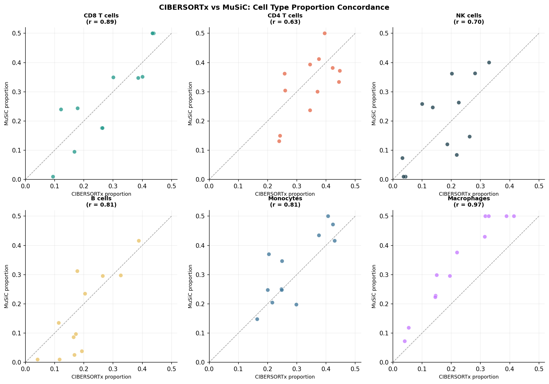
Validating the Proportions
Deconvolution validation follows a hierarchy depending on what ground truth is available.
The strongest validation is comparison against a measured cell type proportion: flow cytometry or mass cytometry (CyTOF) data from the same samples. If your estimated CD8 T cell fraction correlates strongly (r above 0.85) with the flow-measured CD8 fraction across samples, the deconvolution is working. If it does not, your reference may not match your tissue.
When measured proportions are not available, in silico validation uses pseudo-bulk samples with known composition: mix single-cell data from your reference in known proportions and check whether deconvolution recovers those proportions. This tests method accuracy on data that resembles yours without requiring additional experiments.
At minimum, report the estimated proportions alongside the RMSE (for CIBERSORTx) or the weighted RMSE (for MuSiC), inspect the stacked bar plots for biologically implausible values (proportions above 50 percent for a minor cell type, negative proportions before clipping), and check that cells of the same type cluster together in a PCA of the estimated expression profiles.
Reporting Deconvolution in Your Methods Section
Methods text should specify: the tool name and version, the reference used (its source, the number of cell types, whether it was custom or public), the batch correction mode if using CIBERSORTx, and the significance threshold for the CIBERSORTx p-value filter (commonly 0.05). For MuSiC, state the number of subjects contributing cells to the reference and the cell type annotation method.
Example: “Cell type proportions were estimated using CIBERSORTx (version 1.0; Newman et al. 2019) with a custom signature matrix derived from X single-cell RNA-seq data (reference: [source], N cell types). S-mode batch correction was applied because the reference was generated with droplet-based scRNA-seq. Samples with CIBERSORTx p-value above 0.05 were excluded from downstream proportion comparisons.”
Tool Comparison
| Feature | CIBERSORTx | MuSiC |
|---|---|---|
| Interface | Web-based (registration required) | R package |
| Reference input | Signature matrix (pre-built or from scRNA-seq) | Multi-subject scRNA-seq ExpressionSet |
| Handles cross-subject sc variability | Limited | Yes (key design feature) |
| Batch correction between reference and bulk | Yes (B-mode, S-mode) | Not built-in (handled upstream) |
| Works without scRNA-seq reference | Yes (LM22 for immune) | No |
| Cross-condition reference mismatch | Not addressed | MuSiC2 extension addresses this |
| Output includes confidence | p-value per sample | Weighted RMSE |
| Scalability | Limited by web interface | R-based, scales with memory |
| Primary citation | Newman et al. 2019, Nature Methods | Wang et al. 2019, Nature Communications |
| Best suited for | Immune deconvolution, tumor microenvironment | Complex tissues with multi-donor scRNA-seq reference |
NotchBio includes a deconvolution module that accepts a bulk count matrix and a reference signature matrix or single-cell ExpressionSet. If your experiment involves heterogeneous tissue and you want cell type proportions alongside differential expression results, the analysis runs as part of the same pipeline with the same locked parameter record used for the DE analysis.
Related Reading
Further reading
Read another related post
Pathway Enrichment Analysis: GSEA and ORA in R and Python
Pathway enrichment end to end: GSEA and ORA in R with clusterProfiler and fgsea, plus the Python equivalent with gseapy, across MSigDB, KEGG, and GO sets.
BioinformaticsWhy Deterministic Pipelines Beat AI-Generated Ones for RNA-Seq
AI bioinformatics pipelines feel fast until you check the outputs. Here is when to trust AI, when to verify it, and when to use a deterministic platform.
Tutorialfastp vs Trimmomatic vs BBDuk: A Benchmark on RNA-Seq Reads
A side-by-side benchmark of fastp, Trimmomatic, and BBDuk on paired-end RNA-seq data: speed, post-trim quality, mapping rate, and downstream DEG impact.